Preface
In the rapidly evolving landscape of data systems, we often find ourselves gluing together disparate technologies to build a complete platform. We use Redis for caching, Neo4j for graphs, Qdrant or Pinecone for vectors, and Spark for analytics. This fragmentation leads to “Frankenstein” architectures—complex, fragile, and hard to maintain.
Samyama (Sanskrit for “Integration” or “Binding together”) was born from a desire to collapse this complexity.
Since its inception, Samyama has evolved from a high-performance research prototype into a production-ready ecosystem. To serve both the open-source community and the demanding needs of global industry, Samyama is now offered in two editions:
- Community Edition (OSS): The feature-complete, high-performance core for developers and startups.
- Enterprise Edition: Production-hardened with observability, disaster recovery, and advanced optimization for mission-critical workloads.
This book is the story of building Samyama-Graph, a modern, high-performance graph database written in Rust. It is not just a user manual; it is an architectural deep dive. We will peel back the layers to show you how it works—from the byte-level serialization in RocksDB to the lock-free concurrency of our MVCC engine, and up to the distributed consensus algorithms that keep it alive.
Why Rust?
When building a database in the 2020s, the choice of language is pivotal. We chose Rust not just for its hype, but for its promise: Fearless Concurrency.
A graph database is, by definition, a pointer-chasing engine. It demands random memory access patterns that are notoriously hard to optimize and easy to mess up (hello, segmentation faults!). Rust’s ownership model allowed us to implement complex memory management strategies—like Arena Allocation and localized reference counting—without the overhead of a Garbage Collector or the safety risks of C++.
Who is this book for?
- System Architects who want to understand the internals of a modern database.
- Rust Developers curious about real-world patterns for FFI, concurrency, and distributed systems.
- Data Engineers looking for a unified solution for their graph and AI workloads.
Let’s begin the journey.
About the Project & Author
Samyama.ai: The Vision
Samyama Graph is sponsored and developed by Samyama.ai, a company dedicated to building the future of autonomous, hardware-accelerated knowledge systems. Our mission is to unify the fragmented data landscape of graphs, vectors, and optimization into a single “Mechanical Sympathy” engine.
For enterprise inquiries, partnerships, or support, visit our official website: https://samyama.ai
About the Author: Sandeep Kunkunuru
The architecture and implementation of Samyama Graph, as well as this technical guide, are led by Sandeep Kunkunuru.
Sandeep is a specialist in high-performance Rust systems, distributed consensus, and the application of metaheuristic optimization to large-scale graph data. He is the primary maintainer of the Samyama open-source core and the lead architect behind the Enterprise Hardware-Accelerated edition.
Connect with the Project & Author:
- LinkedIn: https://www.linkedin.com/in/sandeepkunkunuru/
- GitHub: https://github.com/samyama-ai/samyama-graph
- Twitter/X: https://x.com/Samyama_AI
Getting Started with Samyama Graph
A step-by-step guide to install, connect, and explore Samyama Graph using the web visualizer at graph.samyama.cloud.
Demo Video
The demo covers: local Samyama Graph setup, connecting graph.samyama.cloud to a local instance, connecting to the hosted endpoint at api.samyama.dev, running Cypher queries, exploring graph visualizations, and using the Schema Explorer and Dashboard.
Option A — Local Setup (Run on Your Machine)
Step 1 — Install Rust
Open your terminal and run:
Mac / Linux
curl --proto '=https' --tlsv1.2 -sSf https://sh.rustup.rs | sh
Windows
- Go to https://rustup.rs
- Download and run
rustup-init.exe - Follow the installer
After installation, restart your terminal. Verify it worked:
rustc --version
cargo --version
Step 2 — Clone the Repository
git clone https://github.com/samyama-ai/samyama-graph
cd samyama-graph
Step 3 — Build the Engine
cargo build --release
When complete you will see:
Finished `release` profile [optimized] target(s) in Xs
Step 4 — Start the Engine
Mac / Linux
./target/release/samyama
Windows
.\target\release\samyama.exe
You will see:
HTTP server starting on port 8080
Server ready. Press Ctrl+C to stop.
The engine is now running on:
- Port 8080 — HTTP API (for the visualizer)
- Port 6379 — Redis protocol (for
redis-cli)
Step 5 — Open the Visualizer
-
Open the Chrome browser
-
Go to graph.samyama.cloud
-
Sign up with your email and password (free)
-
In the connection box, type:
http://localhost:8080 -
Click Connect
You should see:
- Status: healthy ✅
- Version: 1.0.0
- Nodes and Edges count
Note: If you see a
Failed to fetcherror, go to the Chrome address bar → click the lock icon → Site Settings → Insecure Content → set to Allow → refresh the page.
Option B — No Local Setup (Explore Instantly)
If you do not want to install anything:
-
Go to graph.samyama.cloud
-
Sign up with your email and password (free)
-
In the connection box, type:
https://api.samyama.dev -
Click Connect
You are immediately connected to a live Samyama instance with real data. No installation required.
Running Your First Query
-
Click Query Console in the left sidebar.
-
Type this query in the editor:
MATCH (n) RETURN labels(n), count(n) -
Click Run (or press
Ctrl+Enter).
You will see results in the Table tab showing all node types and their counts.
Switch to Graph View
- Click the Graph tab in the results area.
- You will see an interactive force-directed graph:
- Hover over any node to see its properties.
- Drag nodes to rearrange.
- Scroll to zoom in or out.
More Queries to Try
-- See all relationships
MATCH ()-[r]->() RETURN type(r), count(r)

-- Browse nodes with their properties
MATCH (n) RETURN n LIMIT 25

-- Find connected nodes
MATCH (n)-[r]->(m) RETURN n, r, m LIMIT 20
Schema Explorer
The Schema Explorer shows you the complete structure of your graph.
Click Schema Explorer in the left sidebar. You will see:
- Total Nodes — total count across all labels
- Total Edges — total count across all relationship types
- Node Types — each label with its count
- Edge Types — each relationship type with its count
This is useful for understanding what data is in your graph before writing queries.
Dashboard
The Dashboard auto-generates charts from your graph schema — no configuration needed.
Click Dashboard in the left sidebar. You will see panels including:
- Total Nodes — big number card
- Total Edges — big number card
- Node Label Distribution — pie chart
- Edge Type Distribution — pie chart
- Top Labels by Count — bar chart
- Graph Health — connected components, isolated nodes, average degree
Click Open in Console on any panel to see and edit the underlying Cypher query. Every chart is backed by a real Cypher query — you can modify and re-run them in the Query Console.
My Queries (Query History)
All queries you run are automatically saved.
Click My Queries in the left sidebar. You will see three tabs:
- Recent — all queries grouped by date
- Bookmarked — queries you starred
- Frequent — queries you run most often
You can:
- Click Run on any saved query to execute it again
- Click the star icon to bookmark a query
Plan Visualizer
See how the query engine executes your query.
- Click Plan Visualizer in the left sidebar.
- Type a Cypher query.
- Click Explain to see the execution plan as a visual tree.
- Click Profile to see actual execution times per operator.
Common Issues
Failed to fetch on graph.samyama.cloud
Chrome → Lock Icon → Site Settings → Insecure Content → Allow
Port 8080 already in use
lsof -ti :8080 | xargs kill -9
Then restart Samyama.
Build takes too long
The first build normally takes 5–15 minutes on a typical laptop. Subsequent builds are much faster.
No data after connecting
Your graph is empty. Create a sample node:
CREATE (n:Person {name: 'Alice'}) RETURN n
Next Steps
- Read the full documentation: graph.samyama.cloud/book
- Star the repository: github.com/samyama-ai/samyama-graph
- Join the community: Samyama-Graph-OSS-Support WhatsApp Group
- Need help? Message us in the WhatsApp group
That’s it — you’re up and running with Samyama Graph. Happy querying!
Knowledge Graph Catalog
Samyama ships with 8 pre-built knowledge graphs spanning biomedicine, public health, sports, and industrial operations — the 8 packaged snapshots cataloged below total ~8.7M nodes / ~30M edges of curated, open-license content. Each KG is available as a portable .sgsnap snapshot that loads in seconds, stored on S3 (s3://samyama-data/snapshots/) and GitHub Releases, and cataloged in the Supabase kg_registry table.
For the federated mega-benchmark workload — the 8 packaged KGs plus PubMed, OpenFDA FAERS, and OHDSI OMOP — the combined graph reaches ~138M nodes / 1.3B edges across 11 sources. See the Mega Benchmark for the full federated query suite.
Catalog Overview
graph TB
    subgraph "Biomedical Trifecta"
        PKG["🧬 Pathways KG<br/>119K nodes · 835K edges"]
        CTKG["💊 Clinical Trials KG<br/>7.8M nodes · 27M edges"]
        DIKG["💉 Drug Interactions KG<br/>245K nodes · 388K edges"]
    end

    subgraph "Public Health Trifecta"
        DSKG["🦠 Disease Surveillance KG<br/>217K nodes · 241K edges"]
        HDKG["📊 Health Determinants KG<br/>286K nodes · 286K edges"]
        HSKG["🏥 Health Systems KG<br/>20K nodes · 19K edges"]
    end

    subgraph "Sports"
        CKG["🏏 Cricket KG<br/>36K nodes · 1.4M edges"]
    end

    subgraph "Industrial"
        AOKG["🏭 AssetOps KG<br/>781 nodes · 955 edges"]
    end

    PKG -.->|"Gene · Protein"| DIKG
    DIKG -.->|"Drug · Intervention"| CTKG
    DSKG -.->|"Disease · Condition"| CTKG
    DSKG -.->|"Drug · AMR"| DIKG
    DSKG -.->|"Region"| HDKG
    DSKG -.->|"Region"| HSKG

    style CKG fill:#3b82f6,stroke:#333,color:#fff
    style PKG fill:#10b981,stroke:#333,color:#fff
    style CTKG fill:#8b5cf6,stroke:#333,color:#fff
    style DIKG fill:#ec4899,stroke:#333,color:#fff
    style AOKG fill:#f59e0b,stroke:#333,color:#fff
    style DSKG fill:#06b6d4,stroke:#333,color:#fff
    style HDKG fill:#84cc16,stroke:#333,color:#fff
    style HSKG fill:#f97316,stroke:#333,color:#fff
| KG | Nodes | Edges | Labels | Edge Types | Snapshot | Source | Status |
|---|---|---|---|---|---|---|---|
| Cricket KG | 36,619 | 1,392,017 | 6 | 12 | 21 MB | Cricsheet | Live |
| Pathways KG | 118,686 | 834,785 | 5 | 9 | 9 MB | Reactome, STRING, GO | Live |
| Clinical Trials KG | 7,774,446 | 26,973,997 | 15 | 25 | 711 MB | AACT, MeSH, RxNorm | Live |
| Drug Interactions KG | 245,000 | 388,000 | 8 | 9 | 8.1 MB | DrugBank, SIDER, ChEMBL, DGIdb, OpenFDA | Live |
| AssetOps KG | 781 | 955 | 8 | 10 | < 1 MB | Synthetic (AssetOpsBench) | Live |
| Disease Surveillance KG | 216,553 | 241,084 | 6 | 5 | 5.7 MB | WHO GHO | Live |
| Health Determinants KG | 285,635 | 285,628 | 7 | 6 | 6.5 MB | World Bank WDI, WHO Air Quality, WHO WASH | Live |
| Health Systems KG | 19,661 | 19,428 | 3 | 2 | 0.5 MB | WHO SPAR, WHO NHWA | Live |
Cross-KG Federation
The biomedical trifecta (Pathways + Clinical Trials + Drug Interactions) enables queries spanning molecular biology, translational medicine, and pharmacogenomics. With PubMed: 74.3M nodes, 1.07B edges — 96/100 queries pass. BiomedQA benchmark: 98% accuracy with MCP tools.
The public health trifecta (Disease Surveillance + Health Determinants + Health Systems) enables queries from disease outbreaks to population vulnerability to health system capacity — 40/40 queries pass. Bridges to the biomedical trifecta via Country.iso_code, Drug.drugbank_id, and Gene.gene_name.
Together, the 6-KG federation spans molecular biology to population health in a single OpenCypher query. See Cross-KG Federation for details.
Cricket KG
21K international cricket matches from Cricsheet — ball-by-ball data spanning T20, ODI, and Test formats.

Click for full demo (1:56) — Dashboard, Cypher Queries, and Graph Simulation
Schema
graph LR
    Player -->|BATTED_IN| Match
    Player -->|BOWLED_IN| Match
    Player -->|DISMISSED| Player
    Player -->|FIELDED_DISMISSAL| Player
    Player -->|PLAYED_FOR| Team
    Player -->|PLAYER_OF_MATCH| Match
    Team -->|COMPETED_IN| Match
    Team -->|WON| Match
    Team -->|WON_TOSS| Match
    Match -->|HOSTED_AT| Venue
    Match -->|IN_SEASON| Season
    Match -->|PART_OF| Tournament

    style Player fill:#3b82f6,stroke:#333,color:#fff
    style Match fill:#8b5cf6,stroke:#333,color:#fff
    style Team fill:#ef4444,stroke:#333,color:#fff
    style Venue fill:#f59e0b,stroke:#333,color:#fff
    style Tournament fill:#10b981,stroke:#333,color:#fff
    style Season fill:#ec4899,stroke:#333,color:#fff
| Label | Count | Key Properties |
|---|---|---|
| Match | 21,324 | date, match_type, season, winner |
| Player | 12,933 | name |
| Tournament | 1,053 | name |
| Venue | 877 | name, city |
| Team | 383 | name |
| Season | 49 | name |
Example Queries
-- Top 10 run scorers across all formats
MATCH (p:Player)-[b:BATTED_IN]->(m:Match)
RETURN p.name AS player, sum(b.runs) AS total_runs
ORDER BY total_runs DESC LIMIT 10

-- Bowler-batsman rivalries
MATCH (bowler:Player)-[d:DISMISSED]->(victim:Player)
RETURN bowler.name, victim.name, count(d) AS times
ORDER BY times DESC LIMIT 10

-- Venue-team affinity (home advantage)
MATCH (t:Team)-[:WON]->(m:Match)-[:HOSTED_AT]->(v:Venue)
WITH t, v, count(m) AS wins WHERE wins >= 5
RETURN t.name, v.name, wins ORDER BY wins DESC LIMIT 15
Repository: samyama-ai/cricket-kg
Snapshot: kg-snapshots-v1 (cricket.sgsnap, 21 MB)
Pathways KG
Biological pathways knowledge graph combining 5 open-license data sources — Reactome, STRING, Gene Ontology, WikiPathways, and UniProt. Human-only (organism 9606).

Click for full demo (2:06) — Dashboard, Cypher Queries, and Graph Simulation
Schema
graph LR
    Protein -->|PARTICIPATES_IN| Pathway
    Protein -->|CATALYZES| Reaction
    Protein -->|COMPONENT_OF| Complex
    Protein -->|ANNOTATED_WITH| GOTerm
    Protein -->|INTERACTS_WITH| Protein
    Pathway -->|CHILD_OF| Pathway
    GOTerm -->|IS_A| GOTerm
    GOTerm -->|PART_OF| GOTerm
    GOTerm -->|REGULATES| GOTerm

    style Protein fill:#3b82f6,stroke:#333,color:#fff
    style Pathway fill:#10b981,stroke:#333,color:#fff
    style GOTerm fill:#8b5cf6,stroke:#333,color:#fff
    style Reaction fill:#f59e0b,stroke:#333,color:#fff
    style Complex fill:#ef4444,stroke:#333,color:#fff
| Label | Count | Key Properties |
|---|---|---|
| GOTerm | 51,897 | go_id, name, namespace, definition |
| Protein | 37,990 | uniprot_id, name, gene_name |
| Complex | 15,963 | reactome_id, name |
| Reaction | 9,988 | reactome_id, name |
| Pathway | 2,848 | reactome_id, name, source |
| Edge Type | Count | Description |
|---|---|---|
| ANNOTATED_WITH | 265,492 | Protein → GO term annotation |
| INTERACTS_WITH | 227,818 | Protein-protein interaction (STRING, score ≥ 700) |
| PARTICIPATES_IN | 140,153 | Protein → Pathway membership |
| CATALYZES | 121,365 | Protein → Reaction catalysis |
| IS_A | 58,799 | GO term hierarchy |
| COMPONENT_OF | 8,186 | Protein → Complex membership |
| PART_OF | 7,122 | GO term part-of relation |
| REGULATES | 2,986 | GO term regulation |
| CHILD_OF | 2,864 | Pathway hierarchy |
Repository: samyama-ai/pathways-kg
Snapshot: kg-snapshots-v3 (pathways.sgsnap, 9 MB)
Clinical Trials KG
575K+ clinical studies from ClinicalTrials.gov enriched with MeSH disease hierarchy, RxNorm drug normalization, ATC drug classification, OpenFDA adverse events, and PubMed publications.
Schema
graph LR
    ClinicalTrial -->|STUDIES| Condition
    ClinicalTrial -->|TESTS| Intervention
    ClinicalTrial -->|HAS_ARM| ArmGroup
    ClinicalTrial -->|MEASURES| Outcome
    ClinicalTrial -->|SPONSORED_BY| Sponsor
    ClinicalTrial -->|CONDUCTED_AT| Site
    ClinicalTrial -->|REPORTED| AdverseEvent
    ClinicalTrial -->|PUBLISHED_IN| Publication
    ArmGroup -->|USES| Intervention
    Intervention -->|CODED_AS_DRUG| Drug
    Condition -->|CODED_AS_MESH| MeSHDescriptor
    Drug -->|TARGETS| Protein
    Drug -->|CLASSIFIED_AS| DrugClass
    Drug -->|TREATS| Condition
    Gene -->|ENCODES| Protein
    Gene -->|ASSOCIATED_WITH| Condition
    MeSHDescriptor -->|BROADER_THAN| MeSHDescriptor

    style ClinicalTrial fill:#8b5cf6,stroke:#333,color:#fff
    style Condition fill:#ef4444,stroke:#333,color:#fff
    style Intervention fill:#3b82f6,stroke:#333,color:#fff
    style Drug fill:#10b981,stroke:#333,color:#fff
    style Protein fill:#f59e0b,stroke:#333,color:#fff
    style Gene fill:#ec4899,stroke:#333,color:#fff
    style MeSHDescriptor fill:#06b6d4,stroke:#333,color:#fff
    style Publication fill:#84cc16,stroke:#333,color:#fff
| Label | Key Properties | Source |
|---|---|---|
| ClinicalTrial | nct_id, title, phase, overall_status, enrollment | ClinicalTrials.gov |
| Condition | name, mesh_id, icd10_code | ClinicalTrials.gov |
| Intervention | name, type (DRUG/DEVICE/…), rxnorm_cui | ClinicalTrials.gov |
| Drug | rxnorm_cui, name, drugbank_id | RxNorm |
| Protein | uniprot_id, name, function | UniProt |
| Gene | gene_id, symbol, name | Linked ontologies |
| MeSHDescriptor | descriptor_id, name, tree_numbers | MeSH (NLM) |
| Sponsor | name, class (INDUSTRY/NIH/…) | ClinicalTrials.gov |
| Site | facility, city, country, latitude, longitude | ClinicalTrials.gov |
| Publication | pmid, title, journal, doi | PubMed |
| AdverseEvent | term, organ_system, is_serious | OpenFDA |
| ArmGroup | label, type (EXPERIMENTAL/…) | ClinicalTrials.gov |
| Outcome | measure, time_frame, type | ClinicalTrials.gov |
| DrugClass | atc_code, name, level | ATC |
| LabTest | loinc_code, name | LOINC |
Repository: samyama-ai/clinicaltrials-kg (private)
Snapshot: kg-snapshots-v1 (clinical-trials.sgsnap, 711 MB)
Drug Interactions KG
Drug-gene interactions, side effects, indications, bioactivities, and adverse events from 5 open pharmacology databases. Bridges to Pathways KG (via gene name) and Clinical Trials KG (via DrugBank ID).
Schema
graph LR
    Drug -->|INTERACTS_WITH_GENE| Gene
    Drug -->|HAS_SIDE_EFFECT| SideEffect
    Drug -->|HAS_INDICATION| Indication
    Drug -->|HAS_BIOACTIVITY| Bioactivity
    Drug -->|HAS_ADVERSE_EVENT| AdverseEvent
    Drug -->|CLASSIFIED_AS| DrugClass
    Bioactivity -->|BIOACTIVITY_TARGET| Target

    style Drug fill:#ec4899,stroke:#333,color:#fff
    style Gene fill:#3b82f6,stroke:#333,color:#fff
    style SideEffect fill:#ef4444,stroke:#333,color:#fff
    style Indication fill:#10b981,stroke:#333,color:#fff
Performance
- Rust native loader: 245,000 nodes + 388,000 edges in 7.7s
- Snapshot: 8.1 MB (
druginteractions.sgsnap) - BiomedQA benchmark: 98% accuracy with MCP tools
Sources (5 of 6)
| Source | License | Content |
|---|---|---|
| DrugBank CC0 | CC0 | 19,842 drug vocabulary + synonym mappings |
| DGIdb | Open | Drug-gene interactions from 4,182 genes |
| SIDER | CC-BY-SA | Side effects + indications |
| ChEMBL | CC-BY-SA | 208K bioactivity records |
| OpenFDA FAERS | Public | 1.7K adverse event reports |
Repository: samyama-ai/druginteractions-kg
Rust loader: examples/druginteractions_loader.rs in samyama-graph
Snapshot: druginteractions.sgsnap (8.1 MB)
Disease Surveillance KG
WHO Global Health Observatory data — disease case/death counts, vaccine coverage, and health indicators across 234 countries.
Schema
graph LR
    Country -->|IN_REGION| Region
    Country -->|REPORTED| DiseaseReport
    DiseaseReport -->|REPORT_OF| Disease
    Country -->|HAS_COVERAGE| VaccineCoverage
    Country -->|HAS_INDICATOR| HealthIndicator

    style Country fill:#06b6d4,stroke:#333,color:#fff
    style Region fill:#84cc16,stroke:#333,color:#fff
    style Disease fill:#ef4444,stroke:#333,color:#fff
    style DiseaseReport fill:#8b5cf6,stroke:#333,color:#fff
    style VaccineCoverage fill:#f59e0b,stroke:#333,color:#fff
    style HealthIndicator fill:#ec4899,stroke:#333,color:#fff
| Label | Count | Source |
|---|---|---|
| Country | 234 | WHO GHO |
| Region | 6 | WHO regions (AFR, AMR, SEAR, EUR, EMR, WPR) |
| Disease | 15 | Cholera, Malaria, TB, HIV, Meningitis, etc. |
| DiseaseReport | ~49K | Annual case/death counts per country per disease |
| VaccineCoverage | ~10K | DTP3, MCV1, BCG, Polio3 coverage per country per year |
| HealthIndicator | ~164K | Life expectancy, infant mortality, sanitation, water |
Repository: samyama-ai/surveillance-kg
Rust loader: examples/surveillance_loader.rs in samyama-graph
Snapshot: surveillance.sgsnap (5.7 MB)
Data source: WHO GHO OData API — 30 indicators across infectious diseases, vaccines, and health metrics
Health Determinants KG
Population vulnerability indicators from World Bank WDI, WHO Air Quality, and WHO Water/Sanitation — 80 curated indicators across 211 countries (1990–2024).
Schema
graph LR
    Country -->|IN_REGION| Region
    Country -->|HAS_INDICATOR| SocioeconomicIndicator
    Country -->|ENVIRONMENT_OF| EnvironmentalFactor
    Country -->|NUTRITION_STATUS| NutritionIndicator
    Country -->|DEMOGRAPHIC_OF| DemographicProfile
    Country -->|WATER_RESOURCE_OF| WaterResource

    style Country fill:#84cc16,stroke:#333,color:#fff
    style Region fill:#06b6d4,stroke:#333,color:#fff
    style SocioeconomicIndicator fill:#f59e0b,stroke:#333,color:#fff
    style EnvironmentalFactor fill:#ef4444,stroke:#333,color:#fff
    style NutritionIndicator fill:#10b981,stroke:#333,color:#fff
    style DemographicProfile fill:#8b5cf6,stroke:#333,color:#fff
    style WaterResource fill:#3b82f6,stroke:#333,color:#fff
| Category | Nodes | Indicators | Examples |
|---|---|---|---|
| Countries | 211 | — | ISO 3166-1 alpha-3, income level, WB region |
| Regions | 7 | — | South Asia, Sub-Saharan Africa, etc. |
| Socioeconomic | 52,367 | 16 | GDP, GNI, poverty, Gini, unemployment, literacy, health expenditure |
| Environmental | 35,667 | 10 + PM2.5 | PM2.5 exposure, forest area, renewable energy, CO2 |
| Nutrition | 14,073 | 10 | Stunting, wasting, obesity, undernourishment, anemia |
| Demographic | 107,088 | 15 | Population, fertility, life expectancy, infant mortality, urbanization |
| Water | 76,222 | 10 + WASH | Drinking water, sanitation, freshwater withdrawal, water stress |
Performance
- Rust native loader: 285,635 nodes + 285,628 edges in 2.4s
- Snapshot: 6.5 MB (
health-determinants.sgsnap) - Benchmark: 40/40 queries pass (median 15ms)
Sources
| Source | License | Content |
|---|---|---|
| World Bank WDI | CC-BY 4.0 | 80 indicators, 211 countries, 1990–2024 |
| WHO GHO Air Quality | Open | PM2.5 annual mean (1,880 records) |
| WHO GHO WASH | Open | Water/sanitation (47K records) |
Repository: samyama-ai/health-determinants-kg
Rust loader: examples/health_determinants_loader.rs in samyama-graph-enterprise
Snapshot: health-determinants.sgsnap (6.5 MB)
Health Systems KG
Health system capacity — IHR emergency preparedness and health workforce density from WHO, across 233 countries.
Schema
graph LR
    EmergencyResponse -->|CAPACITY_FOR| Country
    HealthWorkforce -->|SERVES| Country

    style Country fill:#f97316,stroke:#333,color:#fff
    style EmergencyResponse fill:#ef4444,stroke:#333,color:#fff
    style HealthWorkforce fill:#3b82f6,stroke:#333,color:#fff
| Label | Count | Source |
|---|---|---|
| Country | 233 | WHO GHO |
| EmergencyResponse | 8,430 | WHO SPAR v2 — 15 IHR capacities per country per year |
| HealthWorkforce | 10,998 | WHO NHWA — physicians, nurses, dentists, pharmacists |
Performance
- Rust native loader: 19,661 nodes + 19,428 edges in 149ms
- Snapshot: 0.5 MB (
health-systems.sgsnap) - Benchmark: 40/40 queries pass (cross-KG with Health Determinants)
Sources
| Source | License | Content |
|---|---|---|
| WHO SPAR v2 | Open | 15 IHR capacity scores, 233 countries |
| WHO NHWA | Open | Health workforce density per 10K population |
Pending sources (loaders built, data not yet downloaded): GAVI vaccine supply, Global Fund disbursements, IHME health expenditure
Repository: samyama-ai/health-systems-kg
Rust loader: examples/health_systems_loader.rs in samyama-graph-enterprise
Snapshot: health-systems.sgsnap (0.5 MB)
AssetOps KG
Synthetic industrial operations graph from the AssetOpsBench benchmark. Models assets, sensors, maintenance schedules, and failure modes for industrial IoT.
| Label | Count | Examples |
|---|---|---|
| Asset | ~200 | Pumps, compressors, turbines |
| Sensor | ~150 | Temperature, vibration, pressure |
| WorkOrder | ~100 | Maintenance tasks |
| FailureMode | ~80 | Bearing failure, seal leak |
| Component | ~100 | Bearings, seals, impellers |
| Location | ~50 | Plants, areas, units |
| Operator | ~50 | Maintenance technicians |
| Schedule | ~50 | Maintenance windows |
Repository: samyama-ai/assetops-kg (private)
Quick Start — Loading Any Snapshot
All snapshots follow the same load pattern:
# 1. Start Samyama Graph (v1.0.0+)
./target/release/samyama

# 2. Create a tenant
curl -X POST http://localhost:8080/api/tenants \
  -H 'Content-Type: application/json' \
  -d '{"id":"TENANT_ID","name":"TENANT_NAME"}'

# 3. Import snapshot into the tenant
curl -X POST http://localhost:8080/api/tenants/TENANT_ID/snapshot/import \
  -F "file=@snapshot.sgsnap"

# 4. Query
curl -X POST http://localhost:8080/api/query \
  -H 'Content-Type: application/json' \
  -d '{"query":"MATCH (n) RETURN labels(n), count(n)","graph":"TENANT_ID"}'

# 5. Explore in Insight
cd samyama-insight && npm run dev
# → http://localhost:5173 (select tenant from dropdown)
# → http://localhost:5173/simulation/TENANT_ID
Note: Use
/api/tenants/:id/snapshot/import(tenant-specific endpoint), NOT/api/snapshot/import. The generic endpoint always loads into the default tenant.
Cross-KG Federation
When multiple knowledge graphs share entity types — the same proteins, drugs, or genes appear in different datasets — loading them into the same Samyama tenant creates a federated graph where a single Cypher query can traverse across data sources.
This chapter shows how to combine the Pathways KG and Clinical Trials KG into a single biomedical graph and answer questions that neither KG can answer alone.
Why Federation?
The Pathways KG knows molecular biology — which proteins interact, what pathways they participate in, which GO processes they’re annotated with. The Clinical Trials KG knows translational medicine — which drugs are in trials, what conditions they treat, what adverse events they cause.
Neither KG alone can answer:
“Which biological pathways are disrupted by drugs currently in Phase 3 trials for breast cancer?”
This query requires traversing:
ClinicalTrial (phase='Phase 3') → STUDIES → Condition (name contains 'breast cancer')
ClinicalTrial → TESTS → Intervention → CODED_AS_DRUG → Drug
Drug → TARGETS → Protein
Protein → PARTICIPATES_IN → Pathway
The first two hops live in the Clinical Trials KG. The last two hops live in the Pathways KG. The Drug → TARGETS → Protein edge is the bridge.
graph LR
    subgraph "Clinical Trials KG"
        CT["ClinicalTrial<br/>(Phase 3)"]
        COND["Condition<br/>(Breast Cancer)"]
        INT["Intervention"]
        DRUG_CT["Drug"]
    end

    subgraph "Bridge Entities"
        DRUG["Drug<br/>(drugbank_id)"]
        PROT["Protein<br/>(uniprot_id)"]
        GENE["Gene<br/>(gene_id)"]
    end

    subgraph "Pathways KG"
        PROT_PW["Protein"]
        PATHWAY["Pathway"]
        GOTERM["GOTerm"]
    end

    CT -->|STUDIES| COND
    CT -->|TESTS| INT
    INT -->|CODED_AS_DRUG| DRUG_CT
    DRUG_CT -.->|"same drugbank_id"| DRUG
    DRUG -->|TARGETS| PROT
    PROT -.->|"same uniprot_id"| PROT_PW
    GENE -->|ENCODES| PROT
    GENE -->|ASSOCIATED_WITH| COND
    PROT_PW -->|PARTICIPATES_IN| PATHWAY
    PROT_PW -->|ANNOTATED_WITH| GOTERM

    style CT fill:#8b5cf6,stroke:#333,color:#fff
    style COND fill:#ef4444,stroke:#333,color:#fff
    style INT fill:#3b82f6,stroke:#333,color:#fff
    style DRUG_CT fill:#10b981,stroke:#333,color:#fff
    style DRUG fill:#10b981,stroke:#333,color:#fff
    style PROT fill:#f59e0b,stroke:#333,color:#fff
    style GENE fill:#ec4899,stroke:#333,color:#fff
    style PROT_PW fill:#f59e0b,stroke:#333,color:#fff
    style PATHWAY fill:#10b981,stroke:#333,color:#fff
    style GOTERM fill:#8b5cf6,stroke:#333,color:#fff
Join Points
Three entity types appear in both KGs with matching identifiers:
| Entity | Pathways KG Property | Clinical Trials KG Property | Join Key |
|---|---|---|---|
| Protein | Protein.uniprot_id | Protein.uniprot_id | UniProt accession (e.g., P04637) |
| Drug | Drug.drugbank_id | Drug.drugbank_id | DrugBank ID (e.g., DB00072) |
| Gene | Gene.gene_id | Gene.gene_id | NCBI Gene ID (e.g., 7157) |
Loading Multiple Snapshots into One Tenant
Step 1: Start the server
./target/release/samyama
Step 2: Create a combined tenant
curl -X POST http://localhost:8080/api/tenants \
  -H 'Content-Type: application/json' \
  -d '{"id":"biomedical","name":"Biomedical (Pathways + Clinical Trials)"}'
Step 3: Load snapshots sequentially
Load the smaller snapshot first, then the larger one. Each import appends to the existing graph — nodes and edges accumulate.
# Pathways first (9 MB, ~119K nodes)
curl -X POST http://localhost:8080/api/tenants/biomedical/snapshot/import \
  -F "file=@pathways.sgsnap"
# Expected: 118,686 nodes, 834,785 edges

# Clinical Trials second (711 MB, ~7.7M nodes)
curl -X POST http://localhost:8080/api/tenants/biomedical/snapshot/import \
  -F "file=@clinical-trials.sgsnap"
# Expected: 7,711,965 nodes, 27,069,085 edges
Step 4: Verify the combined graph
curl -X POST http://localhost:8080/api/query \
  -H 'Content-Type: application/json' \
  -d '{"query":"MATCH (n) RETURN labels(n) AS label, count(n) AS count ORDER BY count DESC","graph":"biomedical"}'
You should see labels from both KGs:
| Label | Source | Expected Count |
|---|---|---|
| ClinicalTrial | Clinical Trials | ~575,000 |
| Condition | Clinical Trials | varies |
| Intervention | Clinical Trials | varies |
| GOTerm | Pathways | 51,897 |
| Protein | Both | 37,990 + Clinical Trials |
| Drug | Both | Clinical Trials + Pathways |
| Gene | Both | Clinical Trials + Pathways |
| Complex | Pathways | 15,963 |
| Reaction | Pathways | 9,988 |
| Pathway | Pathways | 2,848 |
| MeSHDescriptor | Clinical Trials | varies |
| … | … | … |
Important: Snapshot import creates new nodes — it does not merge on matching properties. This means a Protein like TP53 may exist as two separate nodes (one from each snapshot) with the same
uniprot_id. Cross-KG queries must join on properties, not on node identity.
Cross-KG Federated Queries
Since nodes from different snapshots are not merged, cross-KG queries use property-based joins — matching on shared identifiers like uniprot_id or drugbank_id.
Query 1: Pathways disrupted by drugs in Phase 3 breast cancer trials
-- Find drugs in Phase 3 breast cancer trials
MATCH (ct:ClinicalTrial)-[:STUDIES]->(cond:Condition)
WHERE ct.phase = 'Phase 3'
  AND cond.name CONTAINS 'Breast'
WITH ct
MATCH (ct)-[:TESTS]->(int:Intervention)-[:CODED_AS_DRUG]->(drug:Drug)
WITH DISTINCT drug

-- Bridge to pathways via protein targets (property join)
MATCH (drug)-[:TARGETS]->(prot1:Protein)
MATCH (prot2:Protein)-[:PARTICIPATES_IN]->(pw:Pathway)
WHERE prot1.uniprot_id = prot2.uniprot_id

RETURN pw.name AS pathway,
       count(DISTINCT drug.name) AS drugs_targeting,
       collect(DISTINCT drug.name) AS drug_names
ORDER BY drugs_targeting DESC
LIMIT 15
Query 2: GO processes affected by trial drugs
-- Drugs being tested in active trials
MATCH (ct:ClinicalTrial)-[:TESTS]->(int:Intervention)-[:CODED_AS_DRUG]->(drug:Drug)
WHERE ct.overall_status = 'RECRUITING'
WITH DISTINCT drug

-- Bridge to GO annotations via protein targets
MATCH (drug)-[:TARGETS]->(prot1:Protein)
MATCH (prot2:Protein)-[:ANNOTATED_WITH]->(go:GOTerm)
WHERE prot1.uniprot_id = prot2.uniprot_id
  AND go.namespace = 'biological_process'

RETURN go.name AS biological_process,
       count(DISTINCT drug.name) AS drugs,
       count(DISTINCT prot2.name) AS proteins
ORDER BY drugs DESC
LIMIT 10
Query 3: PPI neighbors of clinical drug targets
-- Find proteins targeted by a specific drug
MATCH (drug:Drug {name: 'Trastuzumab'})-[:TARGETS]->(target:Protein)
WITH target

-- Find interaction partners in pathways PPI network
MATCH (pw_prot:Protein)-[:INTERACTS_WITH]-(partner:Protein)
WHERE pw_prot.uniprot_id = target.uniprot_id

RETURN target.name AS drug_target,
       partner.name AS ppi_neighbor,
       count(*) AS interaction_strength
ORDER BY interaction_strength DESC
LIMIT 20
Query 4: Disease ↔ Pathway connections through genes
-- Genes associated with a disease (from clinical trials KG)
MATCH (gene:Gene)-[:ASSOCIATED_WITH]->(cond:Condition)
WHERE cond.name CONTAINS 'Diabetes'
WITH gene

-- Gene's protein → pathways (from pathways KG)
MATCH (gene)-[:ENCODES]->(prot1:Protein)
MATCH (prot2:Protein)-[:PARTICIPATES_IN]->(pw:Pathway)
WHERE prot1.uniprot_id = prot2.uniprot_id

RETURN pw.name AS pathway,
       count(DISTINCT gene.symbol) AS genes,
       collect(DISTINCT gene.symbol) AS gene_list
ORDER BY genes DESC
LIMIT 10
Query 5: Adverse events linked to pathway disruption
-- Drugs with serious adverse events
MATCH (drug:Drug)<-[:CODED_AS_DRUG]-(int:Intervention)<-[:TESTS]-(ct:ClinicalTrial)
MATCH (ct)-[:REPORTED]->(ae:AdverseEvent)
WHERE ae.is_serious = true
WITH drug, count(DISTINCT ae.term) AS ae_count
WHERE ae_count >= 5

-- What pathways do these drugs target?
MATCH (drug)-[:TARGETS]->(prot1:Protein)
MATCH (prot2:Protein)-[:PARTICIPATES_IN]->(pw:Pathway)
WHERE prot1.uniprot_id = prot2.uniprot_id

RETURN drug.name AS drug,
       ae_count AS serious_adverse_events,
       collect(DISTINCT pw.name) AS targeted_pathways
ORDER BY ae_count DESC
LIMIT 10
Testing Instructions
Prerequisites
- Samyama Graph Enterprise v1.0.0+ running on
localhost:8080 - Snapshots downloaded:
pathways.sgsnapfrom kg-snapshots-v3clinical-trials.sgsnapfrom kg-snapshots-v1
- At least 8 GB free RAM (Clinical Trials KG is large)
Step-by-step test script
#!/bin/bash
# test_cross_kg_federation.sh
# Tests cross-KG federation between Pathways and Clinical Trials

set -e
API="http://localhost:8080"

echo "=== Step 1: Create biomedical tenant ==="
curl -s -X POST "$API/api/tenants" \
  -H 'Content-Type: application/json' \
  -d '{"id":"biomedical","name":"Biomedical Federation"}' | python3 -m json.tool

echo -e "\n=== Step 2: Load Pathways KG ==="
curl -s -X POST "$API/api/tenants/biomedical/snapshot/import" \
  -F "file=@pathways.sgsnap" | python3 -c "
import sys,json; d=json.load(sys.stdin)
print(f'  Pathways: {d[\"nodes_imported\"]:,} nodes, {d[\"edges_imported\"]:,} edges')"

echo -e "\n=== Step 3: Load Clinical Trials KG ==="
echo "  (This may take 1-2 minutes for the 711 MB snapshot)"
curl -s -X POST "$API/api/tenants/biomedical/snapshot/import" \
  -F "file=@clinical-trials.sgsnap" | python3 -c "
import sys,json; d=json.load(sys.stdin)
print(f'  Clinical Trials: {d[\"nodes_imported\"]:,} nodes, {d[\"edges_imported\"]:,} edges')"

echo -e "\n=== Step 4: Verify combined graph ==="
curl -s -X POST "$API/api/query" \
  -H 'Content-Type: application/json' \
  -d '{"query":"MATCH (n) RETURN labels(n) AS label, count(n) AS count ORDER BY count DESC","graph":"biomedical"}' | python3 -c "
import sys,json
for r in json.load(sys.stdin)['records']:
    print(f'  {r[0][0]:20s} {r[1]:>10,}')"

echo -e "\n=== Step 5: Check join points ==="

echo "  Proteins with uniprot_id (Pathways):"
curl -s -X POST "$API/api/query" \
  -H 'Content-Type: application/json' \
  -d '{"query":"MATCH (p:Protein) WHERE p.uniprot_id IS NOT NULL RETURN count(p) AS proteins_with_uid","graph":"biomedical"}' | python3 -c "
import sys,json; print(f'    {json.load(sys.stdin)[\"records\"][0][0]:,}')"

echo "  Drugs with drugbank_id:"
curl -s -X POST "$API/api/query" \
  -H 'Content-Type: application/json' \
  -d '{"query":"MATCH (d:Drug) WHERE d.drugbank_id IS NOT NULL RETURN count(d) AS drugs_with_dbid","graph":"biomedical"}' | python3 -c "
import sys,json; print(f'    {json.load(sys.stdin)[\"records\"][0][0]:,}')"

echo -e "\n=== Step 6: Cross-KG query — Pathways disrupted by Phase 3 breast cancer drugs ==="
curl -s -X POST "$API/api/query" \
  -H 'Content-Type: application/json' \
  -d '{
    "query": "MATCH (ct:ClinicalTrial)-[:STUDIES]->(cond:Condition) WHERE ct.phase = '\"'\"'Phase 3'\"'\"' AND cond.name CONTAINS '\"'\"'Breast'\"'\"' WITH ct MATCH (ct)-[:TESTS]->(int:Intervention)-[:CODED_AS_DRUG]->(drug:Drug) WITH DISTINCT drug MATCH (drug)-[:TARGETS]->(prot1:Protein) MATCH (prot2:Protein)-[:PARTICIPATES_IN]->(pw:Pathway) WHERE prot1.uniprot_id = prot2.uniprot_id RETURN pw.name AS pathway, count(DISTINCT drug.name) AS drugs ORDER BY drugs DESC LIMIT 10",
    "graph": "biomedical"
  }' | python3 -c "
import sys,json
d=json.load(sys.stdin)
if 'error' in d:
    print(f'  Error: {d[\"error\"]}')
else:
    print(f'  Columns: {d[\"columns\"]}')
    for r in d.get('records',[])[:10]:
        print(f'    {r}')"

echo -e "\n=== Step 7: Simpler cross-KG validation — shared proteins ==="
curl -s -X POST "$API/api/query" \
  -H 'Content-Type: application/json' \
  -d '{"query":"MATCH (p1:Protein)-[:PARTICIPATES_IN]->(pw:Pathway) MATCH (p2:Protein)<-[:TARGETS]-(d:Drug) WHERE p1.uniprot_id = p2.uniprot_id RETURN count(DISTINCT p1.uniprot_id) AS shared_proteins, count(DISTINCT d.name) AS drugs, count(DISTINCT pw.name) AS pathways","graph":"biomedical"}' | python3 -c "
import sys,json
d=json.load(sys.stdin)
if 'error' in d:
    print(f'  Error: {d[\"error\"]}')
else:
    r=d['records'][0]; print(f'  Shared proteins: {r[0]}, Drugs: {r[1]}, Pathways: {r[2]}')"

echo -e "\n=== Done ==="
Expected results
If both snapshots loaded correctly:
- Label distribution should show labels from both KGs (Pathway, GOTerm, Protein from Pathways; ClinicalTrial, Condition, Intervention from Clinical Trials)
- Join points should show thousands of proteins with
uniprot_idand hundreds of drugs withdrugbank_id - Cross-KG query should return pathways like “Signal Transduction”, “Immune System”, “Disease” that are targeted by Phase 3 breast cancer drugs
- Shared proteins count should be > 0, confirming the bridge works
Troubleshooting
| Issue | Cause | Fix |
|---|---|---|
| Import times out | Clinical Trials snapshot is 711 MB | Increase curl timeout: curl --max-time 600 ... |
| Out of memory | Combined graph needs ~8 GB | Use Mac Mini (16 GB) or reduce to pathways-only |
| Cross-KG query returns 0 rows | Protein IDs don’t overlap | Verify with simpler query: MATCH (p:Protein) WHERE p.uniprot_id = 'P04637' RETURN p |
| Property join slow | No index on uniprot_id | Create index: redis-cli GRAPH.QUERY biomedical "CREATE INDEX FOR (p:Protein) ON (p.uniprot_id)" |
Architecture Notes
Why Property Joins (Not Node Merging)?
Snapshot import creates fresh nodes with auto-assigned IDs. Two Protein nodes from different snapshots with the same uniprot_id are distinct graph nodes. We join them via WHERE p1.uniprot_id = p2.uniprot_id.
Trade-offs:
| Approach | Pros | Cons |
|---|---|---|
| Property join (current) | Simple, no ETL changes, snapshots stay independent | Slower on large joins, duplicate nodes |
| ETL-time merge | Fastest queries, single node per protein | Requires custom loader, order-dependent |
| Post-load MERGE | Clean graph, works with any snapshots | Expensive for millions of nodes |
For production workloads, consider building a dedicated cross-KG ETL that uses MERGE on shared identifiers during loading. For exploration and prototyping, property joins work well.
Future: Native Cross-Tenant Queries
A future Samyama release may support cross-tenant query federation natively, allowing:
-- Hypothetical future syntax
MATCH (drug:Drug)-[:TARGETS]->(p:Protein)
  ON TENANT 'clinical'
MATCH (p2:Protein)-[:PARTICIPATES_IN]->(pw:Pathway)
  ON TENANT 'pathways'
WHERE p.uniprot_id = p2.uniprot_id
RETURN pw.name, drug.name
Until then, loading into a single tenant with property joins is the recommended approach.
Ontology & Standards Catalog
This catalog surveys 147 publicly available ontologies, knowledge graphs, and standards relevant to Samyama Graph’s knowledge graph ecosystem — organized by domain, ranked by relevance tier.
Source of truth:
data/ontology_catalog.csv— machine-readable, importable into any tool or pipeline.
Relevance Tiers
| Tier | Meaning | Count |
|---|---|---|
| 1 — Critical | Directly maps to an active Samyama KG, evaluation workflow, or partner need | 67 |
| 2 — High | Strong alignment; likely needed within 6 months | 61 |
| 3 — Moderate | Useful reference for broader evaluation scenario generation | 20 |
A. Public Health & Epidemiology (31)
Core ontologies for disease classification, surveillance, epidemiology, and LMIC health systems.
| Abbrev | Name | Maintainer | Size | License | Tier |
|---|---|---|---|---|---|
| ICD-11 | International Classification of Diseases | WHO | 55K+ entities | CC BY-ND 3.0 IGO | 1 |
| MeSH | Medical Subject Headings | NLM/NIH | 29K descriptors | Public domain | 1 |
| SNOMED CT | Systematized Nomenclature of Medicine | SNOMED International | 350K+ concepts | Affiliate license | 1 |
| GHO | Global Health Observatory | WHO | 2,300+ indicators | Open access | 1 |
| DHS | Demographic and Health Surveys | USAID/ICF | 400+ surveys, 90+ countries | Open (registration) | 1 |
| GBD | Global Burden of Disease | IHME | 369 diseases, 204 countries | IHME free license | 1 |
| IDO | Infectious Disease Ontology | OBO Foundry | ~3K classes | CC BY 4.0 | 2 |
| OBI | Ontology for Biomedical Investigations | OBO Foundry | ~4.5K classes | CC BY 4.0 | 2 |
| EPO | Epidemiology Ontology | Community (OBO) | ~500 classes | CC BY 4.0 | 2 |
| HL7 FHIR | Fast Healthcare Interoperability Resources | HL7 International | 150+ resources | CC0 1.0 | 2 |
| IHR | International Health Regulations | WHO | 196 parties | Open standard | 2 |
| GLASS | Global AMR Surveillance System | WHO | 127+ countries | Open data | 1 |
| WUENIC | National Immunization Coverage Estimates | WHO/UNICEF | 196 countries | Open data | 1 |
| HPO | Human Phenotype Ontology | Monarch Initiative | 18K+ terms | Custom open | 2 |
| NCIt | NCI Thesaurus | National Cancer Institute | 180K+ concepts | Public domain | 1 |
| PopHO | Population Health Ontology | Univ. of Victoria | ~1K classes | Open | 2 |
| VO | Vaccine Ontology | Univ. of Michigan | ~10K classes | CC BY 3.0 | 2 |
| APOLLO_SV | Apollo Structured Vocabulary | Univ. of Pittsburgh | ~700 classes | CC BY 4.0 | 1 |
| HSO | Health Surveillance Ontology | Data-Driven Surveillance | Emerging | CC BY 4.0 | 1 |
| TRANS | Pathogen Transmission Ontology | Univ. of Maryland | 32 terms | CC0 1.0 | 1 |
| ARO | Antibiotic Resistance Ontology | McMaster Univ./CARD | 5K+ terms | CC BY 4.0 | 1 |
| SYMP | Symptom Ontology | Univ. of Maryland | ~900 terms | CC0 1.0 | 1 |
| NTDO | Neglected Tropical Disease Ontology | UFPE Brazil | 20+ diseases | Open | 1 |
| OMOP CDM | OHDSI Common Data Model | OHDSI | 10M+ concepts | Apache 2.0 | 1 |
| DHIS2 | District Health Information System 2 | Univ. of Oslo | 2.4B+ people served | BSD 3-Clause | 1 |
| OpenMRS | Open Medical Record System | OpenMRS community | 50K+ concepts | MPL 2.0 | 1 |
| WHO DON eKG | WHO Disease Outbreak News KG | Academic (2025) | Decades of reports | Open | 1 |
| ECTO | Environmental Exposures Ontology | OBO Foundry/Monarch | 12K+ classes | CC BY 4.0 | 1 |
| 3M | Micro-Meso-Macro SDOH Ontology | Academic (JMIR) | 383 classes | Open | 1 |
| FHIR SDOH | HL7 FHIR SDOH Profile | HL7 International | Profile/guide | HL7 license | 1 |
| MHO | Mental Health Ontology | Academic consortium | In development | Open | 2 |
B. Social Determinants & Environmental Health (14)
Ontologies mapping environmental exposures, social factors, and their health impacts.
| Abbrev | Name | Maintainer | Size | License | Tier |
|---|---|---|---|---|---|
| WDI | World Development Indicators | World Bank | 1,600+ indicators | CC BY 4.0 | 1 |
| HDI | Human Development Index | UNDP | 191 countries | Open access | 1 |
| ENVO | Environment Ontology | OBO Foundry | ~7K classes | CC BY 4.0 | 1 |
| ExO | Exposure Ontology | OBO Foundry | ~1K classes | CC BY 4.0 | 1 |
| AQD | WHO Air Quality Database | WHO | 6,000+ cities | Open access | 1 |
| AQUASTAT | FAO Water Resources | FAO | 200+ countries | Open access | 1 |
| SDoHO | Social Determinants of Health Ontology | Academic | ~500 classes | Open | 1 |
| ChEBI | Chemical Entities of Biological Interest | EMBL-EBI | 60K+ entities | CC BY 4.0 | 2 |
| TXPO | Toxicology Ontology | OBO Foundry | ~2K classes | CC BY 4.0 | 2 |
| FoodOn | Food Ontology | OBO Foundry | ~30K classes | CC BY 3.0 | 2 |
| SDGIO | SDG Interface Ontology | OBO/UN | ~1.5K classes | CC BY 4.0 | 2 |
| UMEP | Urban Environmental Predictor | Academic | Modular | Open source | 3 |
| GEMS/Water | Global Water Quality | UNEP | 4M+ entries | Open access | 2 |
| CTD | Comparative Toxicogenomics Database | NC State | 2.6M interactions | Open | 2 |
C. Biomedical & Clinical (32)
Disease, drug, genomics, clinical, and anatomy ontologies plus major biomedical knowledge graphs.
| Abbrev | Name | Maintainer | Size | License | Tier |
|---|---|---|---|---|---|
| GO | Gene Ontology | GO Consortium | 47K+ terms | CC BY 4.0 | 1 |
| UMLS | Unified Medical Language System | NLM/NIH | 4.5M+ concepts | UMLS license | 1 |
| DrugBank | DrugBank | OMx/Univ. Alberta | 15K+ drugs | CC BY-NC 4.0 | 1 |
| RxNorm | RxNorm | NLM/NIH | 115K+ concepts | UMLS license | 1 |
| MONDO | Mondo Disease Ontology | Monarch Initiative | 35K+ classes | CC BY 4.0 | 2 |
| DOID | Human Disease Ontology | Univ. Maryland | ~12K classes | CC0 1.0 | 2 |
| LOINC | Lab Observation Identifiers | Regenstrief Institute | 99K+ terms | Free (registration) | 2 |
| ATC | Anatomical Therapeutic Chemical | WHO | 6,300+ codes | WHO license | 2 |
| Hetionet | Hetionet | Himmelstein/UPenn | 47K nodes, 2.25M edges | CC0 1.0 | 2 |
| PrimeKG | Precision Medicine KG | Harvard/Zitnik Lab | 129K nodes, 8M edges | CC BY-NC-SA 4.0 | 1 |
| SPOKE | UCSF Knowledge Engine | UCSF | 27M nodes, 53M edges | API access | 2 |
| PRO | Protein Ontology | Georgetown Univ. | ~40K classes | CC BY 4.0 | 3 |
| SO | Sequence Ontology | OBO Foundry | ~2.5K terms | CC BY-SA 4.0 | 3 |
| FMA | Foundational Model of Anatomy | Univ. Washington | 83K+ classes | Creative Commons | 3 |
| UBERON | Multi-Species Anatomy Ontology | OBO Foundry | 16K+ classes | CC BY 3.0 | 3 |
| CL | Cell Ontology | OBO Foundry | ~2.7K classes | CC BY 4.0 | 3 |
| CDISC | Clinical Data Standards | CDISC | 100+ domains | Free (membership) | 2 |
| ORDO | Orphanet Rare Disease Ontology | INSERM | 10K+ diseases | CC BY 4.0 | 3 |
| PATO | Phenotype and Trait Ontology | OBO Foundry | ~2.7K classes | CC BY 3.0 | 3 |
| DINTO | Drug-Drug Interaction Ontology | Univ. Murcia | ~28K classes | CC BY 3.0 | 1 |
| PharmGKB | Pharmacogenomics KB | Stanford | ~700 drug labels | CC BY-SA 4.0 | 2 |
| OMIM | Online Mendelian Inheritance | Johns Hopkins | ~16.9K entries | Academic free | 2 |
| DisGeNET | Gene-Disease Associations | IMIM Barcelona | 1.1M associations | CC BY-NC-SA 4.0 | 1 |
| Open Targets | Drug Target Platform | EMBL-EBI/Sanger | 63K targets | Apache 2.0/CC0 | 2 |
| Monarch KG | Monarch Initiative KG | NIH | 700K nodes, 7M edges | CC BY 4.0 | 2 |
| Biolink | Biolink Model | Monarch/NIH NCATS | ~300 classes | CC0 1.0 | 1 |
| CKG | Clinical Knowledge Graph | Novo Nordisk/Copenhagen | 16M nodes, 220M rels | MIT | 2 |
| KEGG | Kyoto Encyclopedia | Kanehisa Labs | 560 pathways | Academic free | 2 |
| SIDER | Side Effect Resource | EMBL | 1.4K drugs, 5.9K SEs | CC BY-NC-SA 4.0 | 1 |
| BioKG | AstraZeneca BioKG | AstraZeneca | ~2M entities | MIT | 2 |
| EFO | Experimental Factor Ontology | EMBL-EBI | ~52K classes | Apache 2.0 | 2 |
| KG-Hub | Knowledge Graph Hub | Monarch/LBNL | Multiple KGs | BSD-3 | 3 |
D. AI Safety, Ethics & Evaluation (24)
Risk taxonomies, regulatory frameworks, fairness definitions, and adversarial threat models.
| Abbrev | Name | Maintainer | Size | License | Tier |
|---|---|---|---|---|---|
| AI RMF | NIST AI Risk Management Framework | NIST | 4 functions, 72 subcats | Public domain | 1 |
| EU AI Act | EU AI Act Risk Classification | European Commission | 4 risk tiers | EU regulation | 1 |
| ISO 42001 | AI Management System Standard | ISO/IEC | Clauses + Annex A | Paid standard | 2 |
| ISO 23894 | AI Risk Management | ISO/IEC | Process model | Paid standard | 2 |
| IEEE 7000 | Ethical System Design Standard | IEEE | 10 clauses | IEEE license | 2 |
| MLCommons | AILuminate Safety Benchmark | MLCommons | 12 hazard categories | Open | 1 |
| MIT AIRR | AI Risk Repository | MIT FutureTech | 1,700+ risks | Open access | 1 |
| OWASP AI | AI Security & Privacy Guide | OWASP | 10+ attack categories | CC BY-SA 4.0 | 2 |
| ATLAS | Adversarial Threat Landscape for AI | MITRE | 12 tactics, 30+ techniques | Open | 2 |
| OECD.AI | AI Policy Observatory | OECD | 5 principles | Open access | 2 |
| PAI | Partnership on AI Framework | PAI | Thematic pillars | Open access | 2 |
| Fairness | Fairness-Aware ML Taxonomy | Academic | 20+ definitions | Academic | 1 |
| AIID | AI Incident Database | Responsible AI Collaborative | 3,000+ incidents | Open access | 1 |
| RAI-MM | Responsible AI Maturity Model | Various | 5 maturity levels | Various | 3 |
| ATRS | Algorithmic Transparency Standard | Ada Lovelace Institute | 20+ fields | Open | 3 |
| AI BOM | AI Bill of Materials | NTIA/CISA | Metadata fields | Public domain | 2 |
| AI Atlas Nexus | IBM Graph-Native Risk Ontology | IBM Research | 8+ taxonomies | Apache 2.0 | 1 |
| AIR 2024 | AI Risk Categorization Decoded | Academic (NeurIPS) | 314 risk categories | Open | 1 |
| AILuminate | MLCommons Safety Benchmark | MLCommons | 24K+ prompts/lang | Open | 1 |
| OECD AI Class | AI System Classification | OECD | 5 dimensions | Open access | 1 |
| OWASP LLM | Top 10 for LLM Applications | OWASP | 10 risk categories | CC BY-SA 4.0 | 1 |
| CSET | AI Harm Taxonomy | Georgetown | 10 harm categories | Open | 1 |
| FRIA | Fundamental Rights Impact Assessment | Academic (EU) | Emerging | Open | 2 |
| Fairlearn | Fairness Metrics Toolkit | Microsoft | 10+ metrics | MIT | 1 |
E. Human Rights & Humanitarian (19)
Human rights instruments, humanitarian standards, GBV taxonomies, and crisis data.
| Abbrev | Name | Maintainer | Size | License | Tier |
|---|---|---|---|---|---|
| UDHR | Universal Declaration of Human Rights | UN | 30 articles | Public domain | 1 |
| ICCPR | Intl Covenant on Civil & Political Rights | UN OHCHR | 53 articles | Public domain | 1 |
| UNGPs | UN Guiding Principles on Business & HR | UN OHCHR | 31 principles | Public domain | 1 |
| HXL | Humanitarian Exchange Language | OCHA | 300+ hashtags | Open standard | 1 |
| ReliefWeb | OCHA ReliefWeb Taxonomy | UN OCHA | 100+ terms | Open | 2 |
| Sphere | Sphere Standards | Sphere Association | 4 sectors, 20+ standards | CC BY-NC-ND 4.0 | 2 |
| IHL-Onto | Intl Humanitarian Law Ontology | Academic | ~800 classes | Research | 2 |
| PIM | Protection Incident Classification | UNHCR | 50+ incident types | Open standard | 1 |
| TF-GBV | Tech-Facilitated GBV Taxonomy | HI/Tattle/Academic | 20+ categories | Varies | 1 |
| HSP | Humanitarian Standards Partnership | CHS Alliance | 9 commitments | CC BY-NC-ND 3.0 | 3 |
| CVI | Climate Vulnerability Index | ND-GAIN | 192 countries | Open access | 2 |
| CPO | Conflict and Peace Ontology | UCDP/PRIO | 2.5K+ conflicts | Open access | 2 |
| OntoRights | Human Rights Ontology | Academic | ~500 classes | Open | 1 |
| Uwazi | HURIDOCS Documentation Platform | HURIDOCS | 10K+ templates | Open source | 1 |
| GBVIMS | GBV Information Management System | UNFPA/UNICEF/IRC | 6 GBV types | Open standard | 1 |
| OGBV | Online Gender-Based Violence Ontology | Academic | ~200 classes | Open | 2 |
| CARE | Indigenous Data Governance Principles | GIDA | 4 principles | Open standard | 1 |
| PROV-O | Provenance Ontology | W3C | W3C Recommendation | W3C License | 2 |
| IASC GBV | GBV Guidelines Framework | IASC | Guidelines | Open | 2 |
F–J. Additional Domains
F. Agriculture & Food Security (8)
| Abbrev | Name | Tier |
|---|---|---|
| AGROVOC | FAO Multilingual Agricultural Thesaurus (40K+ concepts, 40+ languages) | 1 |
| CO | CGIAR Crop Ontology (5K+ traits, 30+ crops) | 2 |
| PO | Plant Ontology (~2K classes) | 3 |
| IPC | FAO Food Security Classification (5 phases) | 1 |
| LPO | Livestock Product Ontology | 3 |
| IKO | Indigenous Knowledge Ontology (emerging) | 2 |
| GACS | Global Agricultural Concept Scheme (15K+ concepts) | 2 |
| AgroPortal | Agronomic Ontology Repository (150+ ontologies) | 2 |
G. Accessibility & Disability (6)
| Abbrev | Name | Tier |
|---|---|---|
| WCAG 2.2 | Web Content Accessibility Guidelines (78 success criteria) | 1 |
| ICF | WHO Classification of Functioning & Disability (1,454 categories) | 2 |
| MFOEM | Emotion Ontology (~800 classes) | 2 |
| WAI-ARIA | Accessible Rich Internet Applications (200+ roles) | 2 |
| NCP | Neurodiversity Cognitive Profile Frameworks (emerging) | 2 |
| ISO 9999 | Assistive Technology Classification (11 classes) | 3 |
H. Education & Workforce (5)
| Abbrev | Name | Tier |
|---|---|---|
| ISCED | UNESCO Education Classification (9 levels) | 2 |
| Open Badges | Verifiable Digital Credentials (open standard) | 3 |
| DigComp 2.2 | Digital Literacy Framework (5 areas, 21 competences) | 2 |
| O*NET | Occupational Information Network (1,016 occupations) | 3 |
| ESCO | European Skills & Competences (13.9K skills, 30 languages) | 3 |
I. Legal & Governance (5)
| Abbrev | Name | Tier |
|---|---|---|
| ELI | European Legislation Identifier | 3 |
| LKIF | Legal Knowledge Interchange Format (~200 classes) | 3 |
| GDB | Global Data Barometer (109 countries, 80+ indicators) | 2 |
| DPV | W3C Data Privacy Vocabulary (800+ concepts) | 2 |
| NIST PF | NIST Privacy Framework (5 functions, 18 categories) | 2 |
J. Geospatial & Infrastructure (4)
| Abbrev | Name | Tier |
|---|---|---|
| GeoNames | Geographical Database (12M+ entries) | 2 |
| ISO 3166 | Country Codes (249 countries) | 1 |
| OSM | OpenStreetMap (10B+ features) | 2 |
| Healthsites | Health Facility Locations (160K+ facilities) | 1 |
How These Connect to Samyama KGs
Currently Loaded (code-verified)
graph LR
    subgraph "Samyama KGs"
        PKG["Pathways KG"]
        CTKG["Clinical Trials KG"]
        DIKG["Drug Interactions KG"]
        DSKG["Surveillance KG"]
    end

    subgraph "Loaded via API/Download"
        GO["Gene Ontology<br/>go.json.gz + annotations"]
        Reactome["Reactome<br/>5 data files"]
        STRING["STRING v12<br/>PPI, score≥700"]
        UniProt["UniProt<br/>REST API, human reviewed"]
        WikiP["WikiPathways<br/>.gmt file"]
        MeSH["MeSH<br/>NLM API"]
        RxNorm["RxNorm<br/>rxnav.nlm.nih.gov API"]
        ATC["ATC<br/>from RxNorm properties"]
        OpenFDA["OpenFDA<br/>api.fda.gov"]
        PubMed["PubMed<br/>NCBI E-utilities"]
        DrugBank["DrugBank CC0<br/>vocabulary CSV"]
        DGIdb["DGIdb<br/>interactions TSV"]
        SIDER["SIDER<br/>MedDRA side effects"]
        GHO["WHO GHO<br/>OData API"]
    end

    GO -->|"47K terms"| PKG
    Reactome -->|"pathways"| PKG
    STRING -->|"PPI"| PKG
    UniProt -->|"proteins"| PKG
    WikiP -->|"pathways"| PKG
    MeSH -->|"conditions"| CTKG
    RxNorm -->|"drugs"| CTKG
    ATC -->|"drug classes"| CTKG
    OpenFDA -->|"adverse events"| CTKG
    PubMed -->|"publications"| CTKG
    DrugBank -->|"drug vocab"| DIKG
    DGIdb -->|"drug-gene"| DIKG
    SIDER -->|"side effects"| DIKG
    GHO -->|"indicators"| DSKG

    style PKG fill:#10b981,stroke:#333,color:#fff
    style CTKG fill:#8b5cf6,stroke:#333,color:#fff
    style DIKG fill:#ec4899,stroke:#333,color:#fff
    style DSKG fill:#06b6d4,stroke:#333,color:#fff
Logical Map (full vision including planned)
graph LR
    subgraph "Live KGs"
        PKG["Pathways KG<br/>119K nodes"]
        CTKG["Clinical Trials KG<br/>7.7M nodes"]
        DIKG["Drug Interactions KG<br/>245K nodes"]
        DSKG["Surveillance KG<br/>217K nodes"]
        HDKG["Health Determinants KG<br/>286K nodes"]
        HSKG["Health Systems KG<br/>20K nodes"]
    end

    subgraph "Loaded"
        GO["Gene Ontology"]
        Reactome["Reactome"]
        STRING["STRING"]
        UniProt["UniProt"]
        MeSH["MeSH"]
        RxNorm["RxNorm"]
        ATC["ATC"]
        DrugBank["DrugBank"]
        DGIdb["DGIdb"]
        SIDER["SIDER"]
        GHO["WHO GHO"]
    end

    subgraph "Planned Integrations"
        SNOMED["SNOMED CT"]
        ICD["ICD-11"]
        LOINC["LOINC"]
        UMLS["UMLS"]
        WDI["World Bank WDI"]
        AQUASTAT["FAO AQUASTAT"]
        GAVI["GAVI"]
        SPAR["WHO SPAR"]
    end

    GO --> PKG
    Reactome --> PKG
    STRING --> PKG
    UniProt --> PKG
    MeSH --> CTKG
    RxNorm --> CTKG
    ATC --> CTKG
    DrugBank --> DIKG
    DGIdb --> DIKG
    SIDER --> DIKG
    GHO --> DSKG

    SNOMED -.->|"planned"| CTKG
    ICD -.->|"planned"| DSKG
    LOINC -.->|"planned"| CTKG
    UMLS -.->|"planned"| CTKG
    WDI -.->|"planned"| HDKG
    AQUASTAT -.->|"planned"| HDKG
    GAVI -.->|"planned"| HSKG
    SPAR -.->|"planned"| HSKG

    DSKG -.->|"Region"| HDKG
    DSKG -.->|"Region"| HSKG
    DSKG -.->|"Disease"| CTKG
    DIKG -.->|"Gene"| PKG
    DIKG -.->|"Drug"| CTKG

    style PKG fill:#10b981,stroke:#333,color:#fff
    style CTKG fill:#8b5cf6,stroke:#333,color:#fff
    style DIKG fill:#ec4899,stroke:#333,color:#fff
    style DSKG fill:#06b6d4,stroke:#333,color:#fff
    style HDKG fill:#84cc16,stroke:#333,color:#fff,stroke-dasharray: 5 5
    style HSKG fill:#f97316,stroke:#333,color:#fff,stroke-dasharray: 5 5
Not Yet Loaded
| Ontology | Where Referenced | Status |
|---|---|---|
| SNOMED CT | Clinical Trials test schema | No download or parser code |
| ICD-11 | Catalog description | Not downloaded; ICD-10 codes pass through from AACT but no enrichment |
| LOINC | Schema has LabTest(loinc_code) | No LOINC data loader |
| UMLS | Test schema string | No code at all |
| World Bank WDI | Health Determinants KG (planned) | KG not yet built |
| FAO AQUASTAT | Health Determinants KG (planned) | KG not yet built |
| WHO SPAR | Health Systems KG (planned) | KG not yet built |
| GAVI | Health Systems KG (planned) | KG not yet built |
Data source: data/ontology_catalog.csv — 147 entries across 10 categories.
Real-world Use Cases
Samyama is not just a research project; it is designed to solve complex, real-world problems. We include several fully functional demos in the examples/ directory of the repository.
Here are three key scenarios where Samyama shines.
1. Banking: Fraud Detection
Source: examples/banking_demo.rs
Financial fraud often involves complex networks of transactions that traditional SQL databases struggle to uncover.
The Scenario: A money laundering ring moves illicit funds through a series of “mule” accounts to hide the origin, eventually depositing it back into a clean account. This creates a cycle.
The Solution: We model the data as:
- Nodes:
Account - Edges:
TRANSFER(with propertiesamount,date)
The Query:
MATCH (a:Account)-[t1:TRANSFER]->(b:Account)-[t2:TRANSFER]->(c:Account)-[t3:TRANSFER]->(a)
WHERE t1.amount > 10000
  AND t2.amount > 9000
  AND t3.amount > 8000
RETURN a.id, b.id, c.id
This simple query instantly reveals circular transaction patterns that would require massive, slow JOINs in SQL.
2. Supply Chain: Dependency Analysis
Source: examples/supply_chain_demo.rs
Modern supply chains are fragile. Knowing “who supplies my supplier” is critical for risk management.
The Scenario: A factory produces a “Car”. It needs an “Engine”, which needs “Pistons”, which needs “Steel”. If a strike hits the Steel mill, how does it affect Car production?
The Solution: We use the Graph Algorithms module (specifically Breadth-First Search or custom traversal).
The Logic:
- Start at the “Steel Mill” node.
- Traverse all outgoing
SUPPLIESedges recursively. - Identify all downstream
Factorynodes. - Calculate the “Risk Score” based on the dependency depth.
Developer Tip: You can run this exact scenario locally:
cargo run --example supply_chain_demo. It builds the graph, calculates risks, and outputs a JSON tree of cascading failures.
3. Knowledge Graph: Clinical Trials
Source: examples/clinical_trials_demo.rs + examples/knowledge_graph_demo.rs
Medical research is unstructured. Trials, drugs, and conditions are buried in text documents.
The Scenario: A researcher wants to find “Drugs used for Hypertension that have a mechanism similar to ACE inhibitors.”
The Solution (Graph RAG):
- Ingest: Load ClinicalTrials.gov data into Samyama.
- Embed: Use the “Auto-Embed” pipeline to turn the “Mechanism of Action” text into vectors.
- Query:
- Vector Search: Find drugs with description similar to “ACE inhibitor”.
- Graph Filter:
MATCH (drug)-[:TREATS]->(c:Condition {name: 'Hypertension'}).
4. Smart Manufacturing: Production Optimization
Source: examples/smart_manufacturing_demo.rs
In a modern factory, thousands of variables must be balanced: machine speed, energy cost, and maintenance schedules.
The Solution: Samyama uses its built-in Jaya or GWO (Grey Wolf Optimizer) to adjust production rates across the graph. The objective is to maximize output while keeping total energy consumption below a specific threshold (the constraint).
5. Enterprise SOC: Threat Hunting
Source: examples/enterprise_soc_demo.rs
Security Operations Centers (SOC) deal with millions of events (logins, file access, network traffic).
The Solution: By modeling logs as a graph, security analysts can run Pathfinding algorithms to trace the “Lateral Movement” of an attacker.
- Graph RAG: Use vector search to find “unusual login behavior” semantically similar to known attack patterns.
6. Healthcare: Resource Allocation
Source: examples/clinical_trials_demo.rs (Resource management variant)
Hospitals must constantly balance budget constraints with patient wait times across departments like ER, ICU, and Surgery.
The Solution: Samyama models each department as a node with properties for current staffing (Doctors, Nurses) and equipment (Beds).
- Optimization: Using the Jaya algorithm, Samyama calculates the optimal distribution of 1,000+ staff members across the entire hospital network.
- The Result: Minimize “Total Weighted Wait Time” while ensuring no department falls below “Minimum Staffing” regulations.
7. Social Network Analysis
Source: examples/social_network_demo.rs
Model and analyze social graphs with community detection, influence propagation, and friend-of-friend recommendations. Demonstrates how PageRank and CDLP algorithms identify key influencers and natural communities within large networks.
8. PCA & Dimensionality Reduction
Source: examples/pca_demo.rs
Demonstrates Principal Component Analysis on node feature vectors. Reduces high-dimensional property data (e.g., user profiles with 10+ numeric attributes) down to 2-3 principal components for visualization and clustering. Showcases both the Randomized SVD and Power Iteration solvers.
The Interactive Experience: run_all_examples.sh
To make these use cases accessible, Samyama includes a comprehensive, menu-driven script: scripts/run_all_examples.sh. This script allows users to:
- Build the entire engine and its dependencies.
- Start the Samyama server with a single keystroke.
- Run any of the embedded Rust demos (Banking, Supply Chain, etc.).
- Execute the new Python Client Demo (
examples/simple_client_demo.py), which showcases the high-performance Python bindings over the RESP protocol.
This interactive tool, combined with our Graph Visualizer (scripts/visualize.py), allows developers to see the graph structure and optimization results in real-time, bridging the gap between abstract algorithms and concrete business value.
Mega Benchmark: 500 Queries Across 11 Knowledge Graphs
500 queries. 11 knowledge graphs. 138 million nodes. 1.22 billion edges. One graph, one query language, one server.
Samyama Graph Enterprise v1.0.0 runs the full 500-query mega benchmark across eleven independently-sourced knowledge graphs loaded into a single federated graph — on a single commodity EC2 spot instance.
Headline
500 / 500 pass (100%) — 468 full-pass + 32 data_dependent zero-row matches whose corpus-gap reasons are recorded in the oracle (NCT bridge absent, drug-name casing, no Depression cohort in the OMOP slice, etc.). 0 errors. 0 unexplained empties.
- Total runtime 78 min; query runtime 28 min; load ~50 min
- Six prefixes hit 100% including all three cross-KG categories (XK, PH, MB)
Reproduction caveat: this result was obtained by importing per-KG
.sgsnapfiles via the binary’s startup load path. The HTTP/api/snapshot/importendpoint is capped at 2 GB and cannot ingestpubmed-v2.sgsnap(11 GB) ortrifecta-pubmed.sgsnap(12 GB). Reproducing via the HTTP path requires the body-limit fix tracked in samyama-graph.
The Dataset
| Knowledge Graph | Source | Nodes | Edges | Key Entities |
|---|---|---|---|---|
| PubMed/MEDLINE | NLM | 66.2M | 1.04B | Article, Author, MeSHTerm, Chemical, Journal, Grant |
| Clinical Trials | AACT/ClinicalTrials.gov | 7.8M | 27M | ClinicalTrial, Intervention, AdverseEvent, Site, Sponsor |
| Pathways | Reactome | 119K | 835K | Protein, Pathway, Complex, Reaction, GOTerm |
| Drug Interactions | DrugBank, ChEMBL, SIDER, DGIdb | 245K | 388K | Drug, Gene, SideEffect, Indication, Bioactivity |
| FAERS | FDA Adverse Events | 10.4M | 90M | AdverseEventCase, Reaction, Drug, Outcome |
| UniProt | EBI | 618K | 3.9M | Protein, Organism, GOTerm |
| OMOP | MIMIC-IV (115K patients) | 51.9M | 54M | Person, Visit, ConditionOccurrence, DrugExposure, Measurement |
| Surveillance | WHO SPAR | 217K | 241K | Country, CapacityIndicator |
| Health Determinants | World Bank + WHO | 286K | 286K | Country, SocioeconomicIndicator, EnvironmentalFactor |
| Health Systems | WHO | 20K | 19K | Country, HealthWorkforce, VaccineCoverage |
| NCT Bridge | AACT study_references | — | 747K | REFERENCED_IN (Article → ClinicalTrial) |
| Total | 137.7M | 1.22B |
How the engine clears the workload
Three execution patterns carry the bulk of the 500 queries:
- Adjacency-aware aggregation (ADR-017) —
count(neighbor)over a degree-bounded match set walks per-node adjacency lists rather than scanning every edge. Without this, top-N degree queries time out on PubMed-scale data. - Streaming
WITH … LIMIT—WithBarrierstops scanning upstream after N rows when noORDER BY/WHERE/DISTINCTfollows. Pipeline stages no longer materialize their full input when the next stage only needs a few rows. - Cypher three-valued logic —
IS NOT NULL AND <bool>short-circuits per spec; chainedWHEREclauses AND-combine cleanly. The query author can write what they mean without the engine silently dropping predicates.
Together these shift the bottleneck from engine correctness to corpus coverage. The expected_rows.yaml oracle records each data_dependent empty with a specific corpus reason — so the remaining work is loader, not engine.
What data_dependent covers (32 queries)
These return zero rows but are expected to — the dataset, not the engine, is the constraint:
| Class | Count | Examples |
|---|---|---|
| Drug-name casing | 7 | FAERS uses 'ASPIRIN', DrugBank uses 'Aspirin' — pre-rewrite queries assume one form |
| Loader coverage gaps | 14 | :CODED_AS_DRUG, WaterResource, Bioactivity, HealthWorkforce, SPAR C01 not yet emitted |
| Cohort gaps in slices | ~6 | OMOP slice has no Depression cohort; some MIMIC-IV strata absent in the 115K-patient slice |
| NCT bridge absences | ~5 | Articles without REFERENCED_IN edges to ClinicalTrials in the AACT study_references snapshot |
Infrastructure
| Instance | r7i.16xlarge (64 vCPU, 495 GB RAM) |
| Region | AWS ap-south-1 (Mumbai), spot pricing |
| Disk | 500 GB gp3 |
| Peak memory | ~299 GB (60% utilization) |
| Load time | ~50 min (11 snapshots + NCT bridge + indexes via startup-load path) |
| Query runtime | 28 min |
| Total runtime | 78 min |
| Build | Samyama Graph Enterprise v1.0 |
Reproducing
# On r7i.16xlarge ap-south-1, AMI ami-0d219aaceb19e2c84
./target/release/examples/unified_benchmark \
  --pubmed-snap ~/snapshots/pubmed-v2.sgsnap \
  --ct-snap ~/snapshots/clinical-trials.sgsnap \
  --pw-snap ~/snapshots/pathways.sgsnap \
  --faers-snap ~/snapshots/faers-full.sgsnap \
  --uniprot-snap ~/snapshots/uniprot.sgsnap \
  --omop-snap ~/snapshots/omop-115k.sgsnap \
  --di-snap ~/snapshots/druginteractions.sgsnap \
  --surv-snap ~/snapshots/surveillance.sgsnap \
  --hd-snap ~/snapshots/health-determinants.sgsnap \
  --hs-snap ~/snapshots/health-systems.sgsnap \
  --study-refs ~/study_references.txt \
  --queries ~/benchmark-queries
Snapshots are public at s3://samyama-data/snapshots/. Query CSVs and the raw run output live in this repo under src/data/benchmark/ (benchmark-v100-results.csv).
Hero Run — 187.5M nodes, 1.29B edges, 99% pass (2026-04-30)
Two weeks after the 500/500 mega-benchmark, we ran a larger sweep: a 1000-query corpus against a 187.5M-node / 1.29B-edge graph stitched from the same 11 KGs at full scale (PubMed at 100%, FAERS at full extract, OMOP via Synthea-generated synthetic patients).
| Nodes | 187.5M |
| Edges | 1.29B |
| Queries | 1000-query corpus |
| Pass rate | 99% |
| Instance | AWS r7i-class spot, ap-south-1 |
| Total cost | ~$1.85 |
| Build | Samyama Graph Enterprise v1.0 (pre-merge, hero branch) |
Two engine fixes landed during the run (2026-05-01) and are now in main:
- String-fn NULL-property handling (a small surfaced gap in 3VL coverage).
- Snapshot multi-label index rebuild after import (closed a latent bug when bridge-loading multiple snapshots into one tenant).
The hero run also produced our first cross-KG entity dedup in production — ChEMBL ↔ UniProt joined on the accession property via ADR-019’s import_tenant_with_dedup path.
The hero run is the workload that validates the v1.0 architectural decisions at the scale we care about. The 500-query mega benchmark is the correctness floor (must hit 100% on a curated set); the 1000-query hero run is the stress ceiling (pass rate under real-world noise on a >1B-edge graph).
Biomedical Knowledge Graph Benchmark
100 queries. 4 knowledge graphs. 74 million nodes. 1 billion edges. One query language.
Samyama’s biomedical benchmark demonstrates real-world cross-knowledge-graph queries across the largest open biomedical dataset we know of — unified in a single queryable graph on commodity hardware.
The 100-query workload below is the four-KG biomedical subset. The Mega Benchmark extends it to 500 queries across 11 KGs (adding FAERS, OMOP, UniProt, and the public-health trifecta), with 500/500 passing on the current engine.
The Dataset
| Knowledge Graph | Source | Nodes | Edges | Key Entities |
|---|---|---|---|---|
| PubMed/MEDLINE | NLM | 66.2M | 1.04B | Article, Author, MeSHTerm, Chemical, Journal, Grant |
| Clinical Trials | AACT/ClinicalTrials.gov | 7.8M | 27M | ClinicalTrial, Intervention, AdverseEvent, Site, Outcome, Sponsor, Condition, Drug |
| Pathways | Reactome | 119K | 835K | Protein, Pathway, Complex, Reaction, GOTerm |
| Drug Interactions | DrugBank + ChEMBL + SIDER + DGIdb | 245K | 388K | Drug, Gene, SideEffect, Indication, AdverseEvent, Bioactivity |
| NCT Bridge | AACT study_references | — | 1M+ | REFERENCED_IN (Article → ClinicalTrial) |
| Total | 74.3M | 1.07B |
Results Summary
100 queries executed. 96 returned data. 3 returned empty (specific data not in snapshot). 1 timed out.
| Category | Queries | Pass | Empty | Error |
|---|---|---|---|---|
| PubMed | 35 | 33 | 1 | 1 |
| Clinical Trials | 20 | 19 | 1 | 0 |
| Pathways | 15 | 15 | 0 | 0 |
| Drug Interactions | 15 | 14 | 1 | 0 |
| Cross-KG | 15 | 15 | 0 | 0 |
| Total | 100 | 96 | 3 | 1 |
Infrastructure
- Instance: r6a.8xlarge (32 vCPU, 256 GB RAM, AMD EPYC)
- Cost: ~$2.50 (AWS spot, ap-south-1)
- Import time: 31 minutes from v2 snapshots
- NCT bridge: 1,018,483 REFERENCED_IN edges created in 109 seconds
- Index creation: 10 indexes in ~320 seconds
PubMed Queries (35)
Point Lookups
| ID | Query | Time | Rows | Result |
|---|---|---|---|---|
| PM01 | Article PMID=12345678 | 19.6s | 1 | “Denpasar Declaration on Population and Development” (1994) |
| PM02 | Article PMID=25000000 | 1.3s | 1 | “How to measure technology assessment: an introduction” |
| PM03 | Article PMID=35000000 | 1.3s | 1 | “Hypusinated EIF5A as a feasible drug target…” (2022) |
| PM04 | Article PMID=1 (oldest) | 1.3s | 1 | “Formate assay in body fluids: application in methanol poisoning” |
1-Hop Traversals
| ID | Query | Time | Rows | Result |
|---|---|---|---|---|
| PM06 | Article → Authors | 13.3s | 1 | Arie Hasman |
| PM07 | Article → MeSH terms | 2.4s | 6 | Attitude of Health Personnel, Consumer Behavior, Health Information Systems, Medical Informatics, Technology Assessment |
| PM09 | Article → Journal | 1.3s | 1 | Studies in health technology and informatics |
| PM11 | Author → Articles (reverse) | 1.3s | 10 | Arie Hasman’s publications |
| PM12 | MeSH → Articles | 2.0s | 10 | Articles annotated with “Neoplasms” |
| PM13 | Chemical → Articles | 1.4s | 10 | Articles mentioning “Aspirin” |
| PM14 | Journal → Articles | 1.4s | 10 | Articles in “Nature” |
| PM17 | Articles citing a specific article | 1.3s | 1 | Citation found |
Multi-Hop Analytics
| ID | Query | Time | Rows | Top Result |
|---|---|---|---|---|
| PM15 | Co-authors of an article | 1.3s | 10 | Co-author network for PMID 25000000 |
| PM19 | MeSH co-occurrence (Neoplasms) | 17.5s | 10 | Humans (513,845), Female (138,966), Animals (127,482) |
| PM20 | MeSH co-occurrence (Diabetes) | 6.2s | 10 | Humans (139,986) |
| PM21 | Chemical co-occurrence (Aspirin) | 2.3s | 10 | Platelet Aggregation Inhibitors (12,722) |
| PM22 | Author collaboration network | 1.3s | 10 | Jan Talmon (10 co-authored papers) |
Aggregations
| ID | Query | Time | Rows | Top Result |
|---|---|---|---|---|
| PM23 | Top authors (Smith*) | 32.1s | 10 | Smith Giri (233 papers) |
| PM24 | Most cited articles | 42.7s | 10 | PMID 20000334 (461 citations) |
| PM25 | ML publication trend | 8.4s | 18 | 2020: 4,974 papers |
| PM26 | Top cancer journals | 5.3s | 10 | Cancer (6,059 articles) |
| PM27 | Cancer funding agencies | 3.9s | 10 | NCI NIH HHS (46,137 papers) |
| PM29 | Diabetes funding agencies | 8.7s | 10 | NIDDK NIH HHS (5,123 papers) |
| PM30 | Most published journals | 6.0s | 10 | Nature (140,152 articles) |
| PM31 | Chemical mentions in Nature | 2.3s | 10 | DNA (3,726 mentions) |
| PM32 | MeSH terms for NCI articles | 63.7s | 10 | Humans (438,053) |
| PM35 | ML prolific authors | 5.4s | 10 | Wei Wang (149 papers) |
Clinical Trials Queries (20)
Sample Queries
| ID | Query | Time | Rows | Result |
|---|---|---|---|---|
| CT01 | Trial interventions | 2.2s | 10 | NCT05524376 → no intervention, NCT03092076 → Ticagrelor |
| CT02 | Trial adverse events | 1.6s | 10 | NCT02028182 → Pruritus, NCT03790111 → Nausea |
| CT03 | Trial sites | 1.6s | 10 | Switzerland, Canada, China, Denmark |
| CT05 | Trial sponsors | 1.6s | 10 | Sun Yat-Sen Memorial Hospital |
| CT06 | Trial conditions | 1.6s | 10 | Sepsis |
Aggregations
| ID | Query | Time | Rows | Top Result |
|---|---|---|---|---|
| CT08 | Trials per country | 15.0s | 15 | United States (190,879 trials) |
| CT09 | Most common interventions | 10.1s | 15 | Placebo (41,155 trials) |
| CT10 | Most common adverse events | 16.3s | 15 | Headache (28,130 trials) |
| CT11 | Most studied conditions | 8.2s | 15 | Healthy (10,898 trials) |
| CT12 | Top sponsors | 7.1s | 10 | Assiut University (4,547 trials) |
Complex Queries
| ID | Query | Time | Rows | Top Result |
|---|---|---|---|---|
| CT13 | Cancer trial interventions | 159s | 10 | Placebo (1,597) |
| CT14 | Diabetes trial adverse events | 150s | 10 | Headache (970) |
| CT16 | Condition → Intervention → AE chain | 120s | 10 | Hypertension → Placebo → Headache (116) |
| CT17 | Cancer trial sponsors | 163s | 10 | National Cancer Institute (1,320) |
| CT20 | Multi-arm trials with AE | 142s | 10 | NCT01682876 (4 arms) → Nausea |
Pathways Queries (15)
| ID | Query | Time | Rows | Top Result |
|---|---|---|---|---|
| PW01 | Protein interactions | 9.7s | 10 | IGKV2D-28 → IGHV3-11, IL17A |
| PW03 | Insulin pathways | 1.4s | 9 | Insulin effects on Xylulose-5-Phosphate synthesis |
| PW04 | Protein lookup (TP53) | 1.2s | 1 | TP53 found |
| PW05 | Largest pathways | 1.8s | 10 | Signal Transduction (2,614 proteins), Disease (2,575), Immune System (2,330) |
| PW06 | Most connected proteins | 1.7s | 10 | TP53 (571 interactions) — the “guardian of the genome” |
| PW08 | GO term annotations | 1.4s | 10 | IGKV2D-28 → adaptive immune response |
| PW11 | Pathway hierarchy | 1.4s | 10 | 2-LTR circle formation → Integration of provirus |
| PW14 | Immune system proteins | 1.3s | 20 | Full list |
| PW15 | Protein interaction depth 2 | 1.3s | 10 | 2-hop interaction network from IGKV2D-28 |
Drug Interactions Queries (15)
| ID | Query | Time | Rows | Top Result |
|---|---|---|---|---|
| DI01 | Drug side effects | 1.3s | 10 | Bivalirudin → Abdominal pain, Anaemia |
| DI02 | Drug-gene interactions | 1.3s | 10 | Cetuximab → gene targets |
| DI03 | Drug indications | 1.3s | 10 | Bivalirudin → Haemorrhage |
| DI04 | Drug adverse events | 1.3s | 10 | Cetuximab → adverse events |
| DI06 | Drugs with most side effects | 1.4s | 10 | Pregabalin (839 side effects) |
| DI07 | Most common side effects | 1.5s | 10 | Nausea (985 drugs) |
| DI08 | Drugs sharing gene targets | 1.3s | 10 | Cetuximab ↔ Erythropoietin (shared gene) |
| DI09 | Drugs for diabetes | 1.4s | 10 | Desmopressin → Diabetes insipidus |
| DI13 | Drug indications + side effects | 103s | 10 | Bivalirudin: Haemorrhage (indication) + Abdominal pain (side effect) |
Cross-Knowledge-Graph Queries (15)
These traverse REFERENCED_IN edges connecting 747,505 PubMed articles to clinical trials via PMID↔NCT ID mapping from AACT study_references.
The Headline Results
-- XK02: What drugs are tested in cancer research trials?
-- Spans: MeSH → Article → ClinicalTrial → Intervention (3 KGs)
MATCH (m:MeSHTerm)<-[:ANNOTATED_WITH]-(a:Article)
      -[:REFERENCED_IN]->(t:ClinicalTrial)-[:TESTS]->(i:Intervention)
WHERE m.name = 'Neoplasms'
RETURN i.name, count(DISTINCT t) AS trials ORDER BY trials DESC LIMIT 10
| Intervention | Trials |
|---|---|
| Placebo | 521 |
| Pembrolizumab | 137 |
| Carboplatin | 106 |
| Paclitaxel | 106 |
| Cyclophosphamide | 98 |
Time: 5.2s — Pembrolizumab (Keytruda) is the most-tested non-placebo cancer drug.
-- XK03: What drugs are tested in diabetes research trials?
MATCH (m:MeSHTerm)<-[:ANNOTATED_WITH]-(a:Article)
      -[:REFERENCED_IN]->(t:ClinicalTrial)-[:TESTS]->(i:Intervention)
WHERE m.name = 'Diabetes Mellitus'
RETURN i.name, count(DISTINCT t) AS trials ORDER BY trials DESC LIMIT 10
| Intervention | Trials |
|---|---|
| Placebo | 324 |
| Metformin | 70 |
| Usual care | 50 |
| Insulin | 25 |
| Exercise | 23 |
Time: 2.4s
-- XK04: What adverse events appear in heart disease trials?
MATCH (m:MeSHTerm)<-[:ANNOTATED_WITH]-(a:Article)
      -[:REFERENCED_IN]->(t:ClinicalTrial)-[:REPORTED]->(ae:AdverseEvent)
WHERE m.name = 'Heart Diseases'
RETURN ae.term, count(DISTINCT t) AS trials ORDER BY trials DESC LIMIT 10
| Adverse Event | Trials |
|---|---|
| Headache | 60 |
| Nausea | 56 |
| Syncope | 51 |
| Pneumonia | 49 |
Time: 2.0s
-- XK06: What adverse events appear in Metformin-linked trials?
-- Spans: Chemical → Article → ClinicalTrial → AdverseEvent (4 entities)
MATCH (c:Chemical)<-[:MENTIONS_CHEMICAL]-(a:Article)
      -[:REFERENCED_IN]->(t:ClinicalTrial)-[:REPORTED]->(ae:AdverseEvent)
WHERE c.name = 'Metformin'
RETURN ae.term, count(DISTINCT t) AS trials ORDER BY trials DESC LIMIT 10
| Adverse Event | Trials |
|---|---|
| Headache | 215 |
| Nausea | 207 |
| Nasopharyngitis | 186 |
| Diarrhoea | 185 |
Time: 2.1s — Diarrhoea is a known Metformin side effect, confirmed across PubMed + ClinicalTrials.gov.
All Cross-KG Results
| ID | Query | Time | Rows | Top Result |
|---|---|---|---|---|
| XK01 | Article → Trial links | 39.8s | 10 | PMID 1 → NCT03260829 |
| XK02 | Cancer → Trial interventions | 5.2s | 10 | Pembrolizumab (137 trials) |
| XK03 | Diabetes → Trial interventions | 2.4s | 10 | Metformin (70 trials) |
| XK04 | Heart disease → Trial AE | 2.0s | 10 | Headache (60 trials) |
| XK05 | Aspirin → Trials | 1.5s | 10 | NCT00000491 “Aspirin MI study” |
| XK06 | Metformin → Trial AE | 2.1s | 10 | Headache (215), Diarrhoea (185) |
| XK07 | Cancer trial sites | 3.8s | 10 | US (4,062), China (1,170), France (827) |
| XK08 | NCI-funded → Interventions | 19.4s | 10 | Placebo (933), Lab biomarker (614), Cyclophosphamide (517) |
| XK09 | NCT-linked count | 98.6s | 1 | 747,505 articles linked to trials |
| XK11 | HIV → Trial sites | 11.6s | 10 | US (2,384) |
| XK12 | Alzheimer → Interventions | 2.4s | 10 | Placebo (345) |
| XK13 | NHLBI-funded → Trial AE | 18.3s | 10 | Headache (643) |
| XK14 | Paclitaxel → Trial sponsors | 1.9s | 10 | NCI (64 trials) |
| XK15 | Breast cancer → Outcomes | 4.0s | 1 | 6,591 outcome measures |
What These Results Mean
-
Pembrolizumab dominates cancer trials — The immunotherapy revolution is visible in the data. Across all PubMed articles annotated with “Neoplasms” that link to clinical trials, Keytruda appears in 137 trials, more than any classic chemotherapy agent.
-
Metformin’s GI side effects confirmed cross-database — Diarrhoea ranks 4th in Metformin-linked trial adverse events (185 trials), consistent with clinical knowledge. This was found by traversing Chemical → Article → Trial → AdverseEvent — four entities across two databases.
-
The US conducts 45% of global clinical trials — 190,879 of ~420K total trials. China is second at 1,170 cancer-specific trials.
-
Nature has 140,152 articles in PubMed — making it the most-indexed journal. DNA is its most-mentioned chemical (3,726 articles).
-
TP53 is the most connected protein — 571 interaction partners in Reactome, confirming its role as the “guardian of the genome.”
-
NCI NIH funds 46,137 cancer research papers — and those papers link to 933 placebo-controlled trials.
Query Files
The full query catalog and results are available as CSV for automated benchmarking:
pubmed-queries.csv— 35 PubMed queriesclinical-trials-queries.csv— 20 Clinical Trials queriespathways-queries.csv— 15 Pathways queriesdrug-interactions-queries.csv— 15 Drug Interactions queriescross-kg-queries.csv— 15 Cross-KG queriesverified-results.csv— All 100 results with timings
Reproducing
All knowledge graph snapshots and the benchmark runner are included in Samyama Graph Enterprise Edition. Contact us to access the pre-built snapshots and benchmark tooling.
Public Health Knowledge Graph Benchmark
40 queries. 2 knowledge graphs. 305K nodes. 305K edges. Cross-KG federation with health system capacity data.
The public health benchmark demonstrates Samyama’s ability to load, query, and cross-correlate population health determinants with health system capacity data — answering questions from “Why are populations vulnerable?” to “What capacity exists to respond?”
See also: the public-health KGs are also part of the 11-KG Mega Benchmark federation — the HD/HS/PH prefixes there contribute 40 queries to the 500/500-pass v1.0 result, alongside biomedical, FAERS, OMOP, and UniProt content.
The Dataset
| Knowledge Graph | Source | Nodes | Edges | Key Entities |
|---|---|---|---|---|
| Health Determinants | World Bank WDI + WHO Air Quality + WHO Water/Sanitation | 285,635 | 285,628 | Country, Region, SocioeconomicIndicator, EnvironmentalFactor, NutritionIndicator, DemographicProfile, WaterResource |
| Health Systems | WHO SPAR v2 + WHO NHWA (workforce) | 19,661 | 19,428 | Country, EmergencyResponse, HealthWorkforce |
| Total | 305,296 | 305,056 |
Data coverage:
- 211 countries with World Bank indicators across 5 categories (1990–2024)
- 233 countries with IHR SPAR v2 capacity scores + health workforce density (2020–2023)
- 80 curated WDI indicators: socioeconomic (16), environmental (10), nutrition (10), demographic (15), water (10)
- 1,880 country-year PM2.5 air quality records from WHO GHO
- 47,531 water/sanitation records (safely managed + basic water/sanitation)
- 11,008 health workforce density records (physicians, nurses, dentists, pharmacists)
- 15 IHR capacities: legislation, coordination, financing, laboratory, surveillance, human resources, emergency management, health services, IPC, risk communication, points of entry, zoonotic, food safety, chemical, radiation
Results Summary
40 queries executed. 40 returned data. 0 empty. 0 errors.
| Category | Queries | Pass | Empty | Error | Median (ms) |
|---|---|---|---|---|---|
| Health Determinants | 20 | 20 | 0 | 0 | 27.4 |
| Health Systems | 10 | 10 | 0 | 0 | 12.2 |
| Cross-KG / Cross-Indicator | 10 | 10 | 0 | 0 | 190.7 |
| Total | 40 | 40 | 0 | 0 | 15.1 |
Performance
Infrastructure: MacBook Pro M-series, single process, in-memory graph loaded from .sgsnap snapshots.
| Metric | Value |
|---|---|
| Snapshot import (Health Determinants) | 1.6s (239K nodes, 240K edges) |
| Snapshot import (Health Systems) | 0.1s (8.7K nodes, 8.4K edges) |
| Point lookups | 1.3–4.2 ms |
| Single-hop traversals | 1.8–24.7 ms |
| Aggregation scans | 10.6–133.5 ms |
| Cross-indicator joins | 105–478 ms |
| All 40 queries total | ~3.6s |
Query Categories
Health Determinants (HD01–HD20)
Point lookups, indicator traversals, cross-category analysis, and regional aggregations over World Bank WDI data.
| ID | Name | Time (ms) | Rows |
|---|---|---|---|
| HD01 | Country by ISO code | 4.2 | 2 |
| HD02 | Country by name | 1.9 | 2 |
| HD03 | All regions | 1.3 | 7 |
| HD04 | Countries in a region | 18.1 | 6 |
| HD05 | GNI per capita for India (latest) | 2.2 | 1 |
| HD06 | India poverty rate trend | 2.2 | 5 |
| HD07 | PM2.5 air pollution for India | 1.9 | 5 |
| HD08 | Energy use per capita top 10 | 56.2 | 10 |
| HD09 | Stunting prevalence Nigeria | 2.0 | 5 |
| HD10 | Countries with high stunting (>30%) | 36.7 | 8 |
| HD11 | Population top 10 countries | 133.5 | 10 |
| HD12 | Life expectancy Brazil trend | 2.5 | 10 |
| HD13 | Infant mortality worst countries | 119.9 | 10 |
| HD14 | Water stress high countries | 53.6 | 10 |
| HD15 | Safe drinking water lowest | 59.6 | 10 |
| HD16 | India all indicators for 2022 | 2.3 | 11 |
| HD17 | India environmental profile | 1.9 | 4 |
| HD18 | Poverty vs life expectancy | 478.1 | 10 |
| HD19 | Health expenditure vs infant mortality | 350.9 | 10 |
| HD20 | Regional average GNI per capita | 238.2 | 7 |
Health Systems (HS01–HS10)
IHR SPAR capacity queries — country profiles, rankings, gaps, and trends.
| ID | Name | Time (ms) | Rows |
|---|---|---|---|
| HS01 | Country by ISO code | 1.8 | 2 |
| HS02 | SPAR scores for India | 11.6 | 14 |
| HS03 | SPAR scores for Nigeria | 11.4 | 14 |
| HS04 | Top 10 by surveillance capacity | 10.8 | 10 |
| HS05 | Countries with lowest lab capacity | 11.2 | 10 |
| HS06 | Average SPAR score per country | 12.2 | 10 |
| HS07 | Countries with lowest avg SPAR | 10.6 | 10 |
| HS08 | India SPAR trend over years | 16.0 | 4 |
| HS09 | Risk communication capacity gap (<40) | 12.7 | 10 |
| HS10 | Count countries per SPAR year | 18.0 | 4 |
Cross-KG / Cross-Indicator (PH01–PH10)
Queries spanning multiple indicator categories or joining determinants with health system capacity data.
| ID | Name | Time (ms) | Rows |
|---|---|---|---|
| PH01 | India vulnerability + SPAR capacity | 11.9 | 14 |
| PH02 | High poverty countries SPAR scores | 105.2 | 20 |
| PH03 | PM2.5 vs surveillance capacity | 66.3 | 5 |
| PH04 | Water stress + health expenditure | 274.6 | 10 |
| PH05 | Stunting + infant mortality correlation | 315.6 | 10 |
| PH06 | Urbanization vs life expectancy | 404.6 | 10 |
| PH07 | Under-5 mortality + safe water access | 309.8 | 10 |
| PH08 | Low income full profile + SPAR | 106.1 | 20 |
| PH09 | Health expenditure vs infant mortality | 348.5 | 10 |
| PH10 | Nigeria full determinants profile | 2.0 | 8 |
Sample Query Results
PH02: High poverty countries — do they have health capacity?
MATCH (c1:Country)-[:HAS_INDICATOR]->(pov:SocioeconomicIndicator)
WHERE pov.indicator_code = 'SI.POV.DDAY' AND pov.value > 20
WITH c1.iso_code AS iso, pov.value AS poverty
ORDER BY poverty DESC LIMIT 5
MATCH (e:EmergencyResponse)-[:CAPACITY_FOR]->(c2:Country)
WHERE c2.iso_code = iso AND e.year = 2023
RETURN c2.name, poverty, e.capacity_code, e.score
ORDER BY poverty DESC
This query identifies countries with >20% extreme poverty and correlates with their IHR emergency preparedness scores — answering “Are the most vulnerable populations in countries with the least health system capacity?”
PH07: Under-5 mortality + safe water access
MATCH (c:Country)-[:DEMOGRAPHIC_OF]->(d:DemographicProfile)
WHERE d.indicator_code = 'SH.DYN.MORT' AND d.year = 2022
WITH c, d.value AS u5_mortality
MATCH (c)-[:WATER_RESOURCE_OF]->(w:WaterResource)
WHERE w.indicator_code = 'SH.H2O.SMDW.ZS' AND w.year = 2022
RETURN c.name, u5_mortality, w.value AS safe_water_pct
ORDER BY u5_mortality DESC LIMIT 10
Central African Republic tops both worst lists: 387 under-5 deaths per 1,000 and only 6.1% safely managed drinking water.
6-KG Federation Vision
These two KGs complete the public health trifecta alongside the existing Surveillance KG (217K nodes). Together with the biomedical trifecta (Pathways + Clinical Trials + Drug Interactions), Samyama now supports queries spanning molecular biology to population health:
PUBLIC HEALTH TRIFECTA              BIOMEDICAL TRIFECTA
Surveillance (217K)  ←──────────→  Clinical Trials (7.7M)
         ↓ Country.iso_code               ↑ Drug
Health Determinants (240K)         Drug Interactions (245K)
         ↓ Country.iso_code               ↑ Gene
Health Systems (8.7K) ←─────────→  Pathways (119K)
Bridge property: Country.iso_code (ISO 3166-1 alpha-3) links all public health KGs. Cross-trifecta bridges use Disease.icd_code, Drug.drugbank_id, and Pathogen → Gene mappings.
Data Files
| File | Description |
|---|---|
health-determinants-queries.csv | 20 Health Determinants queries |
health-systems-queries.csv | 10 Health Systems queries |
public-health-cross-kg-queries.csv | 10 Cross-KG queries |
public-health-results.csv | All 40 query results with timing |
Snapshots
Available for download:
| Snapshot | Size | Source |
|---|---|---|
health-determinants.sgsnap | 6.5 MB | GitHub Release kg-snapshots-v6 |
health-systems.sgsnap | 0.5 MB | GitHub Release kg-snapshots-v6 |
| Also on S3 | s3://samyama-data/snapshots/ |
Performance & Benchmarks
Samyama is designed for “Mechanical Sympathy”—aligning software data structures with the physical reality of modern CPU caches and high-speed NVMe storage.
Micro-Benchmarks (Mac Mini M4)
All benchmarks run on Mac Mini M4, 16GB RAM, macOS. Comparison between the Community (CPU-only) and Enterprise (GPU-accelerated via wgpu) builds. For workload-level numbers across the full 11-KG federated dataset (138M nodes, 1.22B edges, 500 queries) see the Mega Benchmark.
Ingestion Throughput
Samyama achieves industry-leading ingestion rates on commodity hardware:
| Operation | CPU-Only (ops/sec) | GPU-Enabled (ops/sec) |
|---|---|---|
| Node Ingestion | 255,120 | 412,036 |
| Edge Ingestion | 4,211,342 | 5,242,096 |
Note: Edge ingestion is significantly faster because it primarily involves appending to adjacency lists and updating the WAL.
Cypher Query Throughput (OLTP)
For transactional workloads, Samyama’s index-driven execution delivers consistent sub-millisecond latencies:
| Graph Scale | Queries/sec | Avg Latency |
|---|---|---|
| 10,000 nodes | 35,360 QPS | 0.028 ms |
| 100,000 nodes | 116,373 QPS | 0.008 ms |
| 1,000,000 nodes | 115,320 QPS | 0.008 ms |
Index-driven lookups achieve O(1) or O(log n) access. QPS is measured with simple MATCH ... WHERE ... RETURN queries on indexed properties.
These numbers demonstrate that Samyama scales almost linearly—throughput at 1M nodes is comparable to 100K because index-based access eliminates full scans.
GPU Acceleration: The Crossover Point
A key finding from these benchmarks is the impact of memory transfer overhead on GPU acceleration.
| Algorithm | Scale (Nodes) | CPU Compute | GPU (inc. Transfer) | Speedup |
|---|---|---|---|---|
| PageRank | 10,000 | 0.6 ms | 9.3 ms | 0.06x (Slowdown) |
| PageRank | 100,000 | 8.2 ms | 3.1 ms | 2.6x |
| PageRank | 1,000,000 | 92.4 ms | 11.2 ms | 8.2x |
Conclusion: For subgraphs smaller than 100,000 nodes, the CPU remains faster. Once the scale exceeds this “crossover point,” the GPU parallelism overcomes the memory transfer cost, leading to massive speedups.
Vector Search (HNSW, k=10)
Vector search utilizes hnsw_rs (CPU) for graph traversal. GPU acceleration in Enterprise is used for batch re-ranking after retrieval.
| Metric (10K vectors, 128-dim) | CPU-Only | GPU Build |
|---|---|---|
| Cosine distance QPS | 15,872/s | 11,311/s |
| L2 distance QPS | 15,014/s | 10,429/s |
| Search 50K vectors | 10,446 QPS | 9,428 QPS |
Note: The slight slowdown in the GPU build for small vector searches is due to the initialization overhead of the GPU context.
GPU at Scale: S-Size Datasets
On LDBC Graphalytics S-size datasets (millions of vertices), the GPU crossover becomes significant:
| Algorithm | Dataset | Vertices | Edges | CPU | GPU | Speedup |
|---|---|---|---|---|---|---|
| LCC | cit-Patents | 3.8M | 16.5M | 9.6s | 4.7s | 2.0x |
| CDLP | cit-Patents | 3.8M | 16.5M | 9.5s | 11.1s | 0.85x |
| PageRank | datagen-7_5-fb | 633K | 68.4M | — | CPU fallback | — |
Note: Extremely dense graphs (e.g., 68M edges on datagen-7_5-fb) trigger CPU fallback due to the 256MB GPU buffer limit on Apple Silicon. Dedicated GPUs with larger VRAM can handle these datasets.
LDBC Graphalytics Validation
Samyama has achieved 100% validation against the LDBC Graphalytics benchmark suite—the industry standard for graph analytics correctness:
| Algorithm | XS Datasets (2) | S Datasets (3) | Total |
|---|---|---|---|
| BFS | ✅ 2/2 | ✅ 3/3 | 5/5 |
| PageRank | ✅ 2/2 | ✅ 3/3 | 5/5 |
| WCC | ✅ 2/2 | ✅ 3/3 | 5/5 |
| CDLP | ✅ 2/2 | ✅ 3/3 | 5/5 |
| LCC | ✅ 2/2 | ✅ 3/3 | 5/5 |
| SSSP | ✅ 2/2 | ✅ 1/1 | 3/3 |
| Total | 12/12 | 16/16 | 28/28 |
S-size datasets include cit-Patents (3.8M vertices), datagen-7_5-fb (633K vertices, 68M edges), and wiki-Talk (2.4M vertices). All results match LDBC reference outputs exactly.
Developer Tip: Run the validation yourself with
cargo bench --bench graphalytics_benchmark. LDBC datasets are available indata/graphalytics/.
LDBC SNB Interactive & BI Workloads
Beyond Graphalytics (which validates algorithm correctness), Samyama includes benchmark harnesses for the LDBC Social Network Benchmark (SNB) — the industry-standard workload for graph database query performance.
SNB Interactive Workload
21 queries adapted for Samyama’s OpenCypher engine, plus 8 update operations:
| Category | Queries | Description |
|---|---|---|
| Interactive Short | IS1–IS7 | Point lookups: person profile, posts, friends |
| Interactive Complex | IC1–IC14 | Multi-hop traversals: friend-of-friend, common interests, shortest paths |
| Insert Operations | INS1–INS8 | Concurrent writes: new persons, posts, comments, friendships |
cargo bench --bench ldbc_benchmark                    # All 21 queries
cargo bench --bench ldbc_benchmark -- --query IC6     # Single query
cargo bench --bench ldbc_benchmark -- --updates       # Include writes
SNB Business Intelligence (BI) Workload
20 complex analytical queries testing OLAP-style aggregation over the social network graph:
| Category | Queries | Description |
|---|---|---|
| BI Queries | BI-1 to BI-20 | Heavy aggregation, multi-hop analytics, temporal filtering |
Note: Several BI queries require features beyond current OpenCypher coverage (APOC, CASE, list comprehensions). These are adapted to simplified Cypher that captures the analytical intent using supported constructs.
cargo bench --bench ldbc_bi_benchmark
cargo bench --bench ldbc_bi_benchmark -- --query BI-1
Both workloads operate on the LDBC SF1 dataset loaded via cargo run --example ldbc_loader.
LDBC FinBench Workload
Samyama also includes a harness for the LDBC Financial Benchmark (FinBench) — modeling financial transaction networks with accounts, persons, companies, loans, and mediums.
| Category | Queries | Description |
|---|---|---|
| Complex Reads | CR1–CR12 | Multi-hop fund transfers, blocked account detection, loan chains |
| Simple Reads | SR1–SR6 | Account lookups, transfer history, sign-in records |
| Read-Writes | RW1–RW3 | Mixed read-write transactions |
| Writes | W1–W19 | Account creation, transfers, loan operations |
40+ queries total, covering both OLTP and analytical patterns for financial graph workloads.
cargo bench --bench finbench_benchmark
cargo bench --bench finbench_benchmark -- --query CR-1
cargo bench --bench finbench_benchmark -- --writes    # Include write operations
Data is loaded via cargo run --example finbench_loader, which can generate synthetic FinBench-compatible datasets.
The Power of Late Materialization
One of our most impactful architectural choices remains Late Materialization.
Latency Impact (1M nodes)
| Query Type | Latency (Before) | Latency (After) | Improvement |
|---|---|---|---|
| 1-Hop Traversal | 164.11 ms | 41.00 ms | 4.0x |
| 2-Hop Traversal | 1,220.00 ms | 259.00 ms | 4.7x |
Bottleneck Analysis
Profiling our query engine reveals a shift in where time is spent:
| Component | Time | % of 1-Hop |
|---|---|---|
| Parse (Pest grammar) | ~22ms | 54% |
| Plan (AST → Operators) | ~18ms | 44% |
| Execute (Iteration) | <1ms | 2% |
Conclusion: The actual execution of the graph traversal is sub-millisecond. The remaining overhead is in the language frontend (parsing and planning). Our roadmap includes AST Caching and Plan Memoization to bring warm-query latency down to the ~10ms range.
Note: These timings reflect cold-start conditions (first query execution). Subsequent queries benefit from OS-level page cache and instruction cache warmth, reducing total latency significantly.
Cross-Engine Benchmarks
Measured against Neo4j 5, Memgraph and FalkorDB. Every figure here is first-party — Samyama and the competitor measured through the same harness and, for LDBC, on the same host. That distinction is the point of the page, because the comparison numbers quoted in the FAQ are taken from competitors’ own published benchmarks, run on their hardware and their configuration.
Where these live, and why not in the open repo. Cross-engine runs depend on competitor configurations and the licence terms those runs are performed under, so they are maintained in the private
samyama-graph-competitor-benchmarksrepo and published selectively rather than continuously. The rule the engine applies: a number a reader can reproduce belongs next to the code that produces it; a number that required another vendor’s licensed software to obtain does not. A consequence worth stating: you cannot open the artifacts behind this page. Each figure below names the run it came from so it can at least be asked for by name.
LDBC SNB Interactive at SF10 — three engines, one host
Samyama, Neo4j 5 and FalkorDB on a single AWS r6a.8xlarge (2026-08-29):
| Result | |
|---|---|
| Complex reads within 5× of the best competitor | 14 of 14 |
| Worst complex read | IC11 at 2.77× |
| Faster than both competitors | 7 of 14 |
The short reads are not clean, and that is the honest half of this
section. They are the bar for the PERF-04 requirement and they fail it:
IS3 at 7.41× and IS1 at 2.78×. That is a measured failure rather than
an unmeasured one, which is the only thing to be said in its favour.
Two earlier runs of this benchmark are superseded and should not be requoted: 2026-08-19 (12 of 14 within 5×, IC6 timing out, IC11 at 11.5×, against Neo4j alone) and 2026-08-23 (13 of 14, IC11 at 9.4×). The progression is real, but quoting the old IC11 figure understates the engine by 4×, and quoting the old “85–170× slower on complex reads” figure is worse still — that one came from a run whose Samyama and competitor columns were measured on different machines.
Cypher conformance — openCypher TCK
One scenario list, one comparator, a per-engine driver that only executes and renders. The two columns are different runs on different corpora, so each carries its own provenance rather than implying a single measurement:
| Engine | 1,244-scenario set (2e13f46, 2026-08-20) | 3,766-scenario set (7708d60) |
|---|---|---|
| Samyama | 85.0% | 97.0% |
| Neo4j 5 | 98.9% | 79.4% |
| Memgraph | 89.8% | 65.9% |
| FalkorDB | 89.1% | 65.7% |
Read both columns. On the narrower set Samyama trails Neo4j by 13.9 points; on the wider one it leads by 17.6. The project’s own rule about the first column is blunt: 85% must never be quoted alone, because the gate it satisfies has two halves and only one is met — the absolute ≥85% bar passes with three scenarios of margin, while “within 5 points of the best competitor” needs 93.9%.
Every engine falls on the wider corpus, and Neo4j falls nearly twenty points. That is itself the evidence the expansion is sound rather than malformed: a corrupted corpus would have collapsed a mature engine to something implausible, not to 79.4%.
The Samyama figure on the wider set reads 97.0% here and 97.3% in the engine’s own-engine record. Both are right: the cross-engine comparison scores 3,766 scenarios through the judge path, the direct run evaluates 3,762. The judge figure is the one to compare against a competitor, because that is how the competitors were scored.
Scope, because this number is easy to over-quote. This is conformance, not performance and not scale. The competitor figures are one run of one container image each from 2026-08-24 — a fixed baseline, not a live measurement. Kuzu is absent: it is schema-first, so the TCK’s schema-free fixtures do not load. Four engines are not the field.
Hierarchy queries — and what the comparison leaves out
Against Neo4j on an identical graph, 94× across the 58 queries expressible on both engines.
That number is true and it is also a selection effect, which the earlier version of this chapter did not say. The 58 queries expressible on both engines are exactly the classes the index wins — H1, H2, H3, H5, H10. H4, H6 and H7 cannot be written in Neo4j at all, so the three classes where the index loses are absent from the 94× comparison by construction. That is what “expressible on both” means; it is not a rigged selection, but leaving it unsaid turns a scoped result into a general claim.
What the full corpus says, over the same 108 queries:
| Measure | Value |
|---|---|
| Ratio of medians | 2.56× faster |
| Geometric mean | 1.88× |
| Total corpus time | 0.45× — the corpus takes 2.2× longer |
All three are true, and for a long time only the first was published. 34 of 108 queries are slower with the index, three classes by close to an order of magnitude: H7 lowest-common-ancestor 0.09×, H4 cross-hierarchy conjunction 0.21×, H6 anti-subsumption 0.49×. So the index does not pay for itself across its own corpus; it pays enormously on the shapes it was built for.
Two further caveats on the cross-engine figure itself: without the hierarchy index, Samyama is 1.6× slower than Neo4j on the same set, so the index is the differentiator rather than the engine. And H9’s apparent speedup is withdrawn — it has no independent baseline, because the baseline arm removes the very index its query requires.
What makes H2 and H10 win by orders of magnitude is that roll-up latency is flat in subtree size: 16.0 ns at one node, 16.6 ns at 137,257.
What this page is not
Each section is one suite’s result. Where the product stands across the whole
requirement set — met, blocked, unmeasured, or measured only by proxy — is
recorded in SCORECARD.json, assembled by the conformance harness from run
envelopes. The count and the breakdown move with every run, so they are
deliberately not transcribed here; the file is the source of truth. It lives
with the cross-engine results, in the private repo, for the same reason they
do.
Engine Layers — Schema, Data, Statistics, Cache
A database is not one thing; it is four things layered on top of each other. This chapter names the four layers Samyama’s engine works with, explains what each one is for, and maps them to what already exists in the codebase and what is planned.
The rest of Part III (Query Engine, Query Optimization, Persistence, Managing State, etc.) walks each layer in detail. This chapter is the map.
The four layers
graph TB
    L3["<b>Layer 3 — Cache</b><br/>parameterised-query result cache<br/><i>hash(query, params) → rows, TTL</i>"]
    L2["<b>Layer 2 — Statistics</b><br/>cardinalities, distributions, histograms<br/><i>drives plan selection</i>"]
    L1["<b>Layer 1 — Data</b><br/>nodes, edges, properties, labels<br/><i>the graph itself</i>"]
    L0["<b>Layer 0 — Schema / Metadata</b><br/>labels, edge types, property keys, indexes<br/><i>what the shape of the data is</i>"]

    L3 --> L2 --> L1 --> L0

    style L0 fill:#4a9eff,stroke:#333,color:#fff
    style L1 fill:#51cf66,stroke:#333,color:#fff
    style L2 fill:#ffd43b,stroke:#333
    style L3 fill:#b197fc,stroke:#333,color:#fff
Read the arrows as “depends on”. A cache entry (Layer 3) references data (Layer 1); statistics (Layer 2) summarise the data; the data is described by the schema (Layer 0).
Each layer changes at its own pace, and each has its own API surface.
| Layer | Changes at speed of… | Analogue in Postgres | Analogue in Neo4j |
|---|---|---|---|
| 0 — Schema | slow (create/alter DDL) | information_schema.* | db.schema.* |
| 1 — Data | fast (every write) | table rows | nodes and relationships |
| 2 — Statistics | periodic (ANALYZE, or after N writes) | pg_statistic | db.stats.* |
| 3 — Cache | short-lived (per query, TTL) | no first-class equivalent (external, e.g. pgpool-II query cache) | no first-class equivalent (external caching layer / APOC) |
Layer 0 — Schema / Metadata
What it is. The set of labels, edge types, property keys, and indexes that describe the shape of the data — not the data itself. If someone asks “what kinds of things does this graph hold?”, the answer lives at Layer 0.
Why it needs a first-class API. Every mature relational database has an
information_schema — you can ask “how many tables?”, “what columns does this table have?”,
“what indexes exist?” without touching a single row. That capability is what tools like
IDEs, migration frameworks, MCP tool-generators, and query planners depend on. A graph
database needs the same.
Graph schema is different from relational schema in one important way: it is fluid.
In Postgres you ALTER TABLE before you can insert into a new column. In a property graph,
a CREATE (:NewLabel {new_property: 42}) is legal without any prior DDL — the label and
the property key spring into existence with the write. So the schema changes, just more
slowly than the data does. Layer 0 has to track that fluid evolution.
Where it lives in samyama-graph today: src/graph/catalog.rs (GraphCatalog) holds
distinct labels, edge types, and per-label/per-type counts derived from the data. It is
rebuilt on bulk load and on snapshot import (samyama-graph#340, #8).
GraphCatalogserves two layers. The schema entries — the set of labels and edge types — are Layer-0 metadata. The per-label / per-edge-type counts on the same struct are the first pieces of Layer 2 (statistics), consumed by the cost model. Both layers read from the same catalog because the shape and the cardinality of the data live naturally in the same place; the layers are distinguished by what is read, not by where it is stored. Layer 2 below adds histograms and other summaries on top.
What ships today at the Cypher level: CALL db.schema.visualization() — returns a
schema-shape summary usable by tools and UIs.
Gaps to fill (Layer-0 backlog):
- Sister procedures beyond
visualization—CALL db.schema.labels(),db.schema.edgeTypes(),db.schema.propertyKeys(:Label), and their multi-tenant siblings. Today the rest of this data is only reachable via bespoke HTTP endpoints, not via Cypher. - Property-type inference (e.g. “Trial.phase is a string enum of {NA, Phase1, …}”) — the
MCP tool generator in
sdk/python/samyama_mcpre-derives this on every start; it should live in the catalog. - Access control at the schema level (RBAC) — deferred, but the API surface for it belongs on Layer 0.
Layer 1 — Data
What it is. The nodes, edges, and their properties. This is what you read and write with Cypher.
Where it lives: src/graph/ — GraphStore, Node, Edge, PropertyValue, adjacency
lists, columnar property store (ADR-021). Nothing else in the engine holds authoritative
data; every other layer either describes it (Layer 0), summarises it (Layer 2), or
memoises answers about it (Layer 3).
How it is persisted: RocksDB + WAL when persistence is enabled; snapshots via .sgsnap
format for point-in-time export/import. See Persistence at Scale and Managing State
(MVCC & Memory) for the mechanics.
What Layer 1 is not: it is not the place for materialised aggregates, statistics, or cached query results. Those all live above. Keeping Layer 1 authoritative and slim is what makes rebuilding everything above it well-defined.
Layer 2 — Statistics
What it is. Summary numbers about Layer 1 that the query planner reads to choose a plan. Row counts per label, edge-type frequencies, in/out-degree distributions, property histograms, distinct-value estimates.
Why they matter. Consider a two-way join between a table (or subgraph) with 100 million rows and one with 100 rows. If the planner knows the smaller side is small, it will hash it and probe the big one — millisecond query. If it treats both sides as opaque, it might scan the big side once per row of the small side — hours. This decision is entirely on the back of statistics. Without them, a cost-based planner has nothing to be cost-based about.
Where it lives in samyama-graph today:
- Storage:
src/graph/catalog.rs(GraphCatalog) — the same struct that carries Layer 0’s schema also carries the cardinality counts that this layer consumes (see the callout under Layer 0). This is the “triple statistics” fixed bysamyama-graph#340and#8on bulk load and snapshot import. - Consumer:
src/query/executor/cost_model.rs— reads catalog cardinalities inestimate_label_scan,estimate_expand_in, andestimate_expand_outto score candidate plans. See Query Optimization (Explain) and Picasso — Plan-Space Visualisation for the plan-space enumeration and the reduction-factor metric.
Known gap (well-scoped): property histograms are not yet built. Range and inequality
predicates (WHERE t.date > '2024-01-01', WHERE n.age > 30) fall back to the default
selectivity constants documented in
Picasso — Plan-Space Visualisation (0.33 for range,
0.1 for inequality). Because these are constants, the Picasso parameter-sweep
heatmap for such a predicate is uniformly flat — the estimated cost does not respond to
the parameter value. This is the QP-06 item on the query-planner backlog and it is the
single biggest opportunity to improve plan
quality on filtered scans.
Refresh cadence: today Layer 2 is rebuilt at bulk load / snapshot import time (#340,
#8). It is not yet incrementally maintained during small writes — a background
“analyze” pass is the natural next step once histograms land, so the two changes are
usually planned together.
Layer 3 — Cache
What it is. Memoised results of previously-executed queries, keyed by the query text plus its parameter values. On a cache hit, the engine returns the stored rows without re-planning or re-executing.
Why not another in-memory cache layer? Samyama is already an in-memory database. Stacking a second in-memory cache (Redis-style) on top of an in-memory DB just doubles the RAM footprint for the same data with no latency win. Instead, Layer 3 lives inside the graph itself — cache entries are ordinary nodes/edges under a system-owned tenant or a reserved subgraph, with their own TTL.
Key discipline: fully-parameterised or nothing. A cache entry is only safe when the
query is fully parameterised — the query text and every value it depends on are known.
A query with a literal Virat Kohli in it and a query with $name = "Virat Kohli" are
the same execution, but only the second one can be safely hashed for cache lookup, because
the first collides with any other literal that happens to look identical.
Contract:
- Key:
hash(canonical_query_text, params, tenant, graph). - Value: the
QueryResult(columns, records, referenced nodes/edges). - TTL: every entry has an expiry timestamp. There is no “cache forever.”
- Eviction: a lightweight sweeper walks expired entries and removes them.
- Multi-tenant migration: because cache entries live in the graph, they can be moved between shards / tenants based on where memory is cheapest at the moment. This is a future capability of Layer 3, not a shipping one — but the storage shape makes it easy.
Status: Layer 3 (result cache) is a design decision from the Aug-14 discussion; the storage shape above is the target, and no implementation ships yet.
Not to be confused with the compiled-plan cache. The engine already has a
PlanCacheEntryatsrc/query/executor/planner.rs:397that memoises the chosen plan (index hint, timestamp) per query hash — that’s a Layer-2/3-boundary optimisation and avoids re-planning, but it does not avoid re-executing. Layer 3 as described here is the larger step: memoise the result rows keyed by query + params, so a hit skips execution entirely.
How the four layers cooperate on a query
sequenceDiagram
    participant C as Client
    participant L3 as Layer 3 (Cache)
    participant P as Planner
    participant L2 as Layer 2 (Stats)
    participant L0 as Layer 0 (Schema)
    participant L1 as Layer 1 (Data)

    C->>L3: MATCH (t:Trial {country:'India'}) RETURN t.trial_id
    alt cache hit
        L3-->>C: cached rows
    else cache miss
        L3->>P: parse + plan
        P->>L0: is 'Trial' a real label? 'country' a real property?
        P->>L2: how many Trials? how selective is country='India'?
        L2-->>P: 363K trials, ~10% match
        P-->>P: pick plan (IndexScan + Filter vs full scan)
        P->>L1: execute chosen plan
        L1-->>P: rows
        P-->>L3: store (query, params, rows, TTL)
        L3-->>C: rows
    end
Every layer is queried once per query, in that order. When statistics are missing (Layer 2 gap), the planner picks the wrong plan. When schema is stale (Layer 0 gap), the planner either errors out or falls back to a scan. When cache is absent (Layer 3 not yet built), you pay the full plan + execute cost every time.
Implementation status
| Layer | Component | Status |
|---|---|---|
| 0 | GraphCatalog (labels, edge types, per-label counts) | Implemented (src/graph/catalog.rs) |
| 0 | Rebuild after bulk load / snapshot import | Implemented (samyama-graph#340, #8) |
| 0 | CALL db.schema.visualization() | Implemented (src/query/executor/planner.rs, operator.rs) |
| 0 | Other db.schema.* procedures (labels, edgeTypes, propertyKeys(:Label)) | Planned — samyama-graph-enterprise#534 |
| 0 | Property-type / enum inference in catalog | Planned (today re-derived by MCP generator) — enterprise#535 |
| 0 | Schema-level RBAC | Deferred (no issue yet — untimed) |
| 1 | GraphStore, columnar property store (ADR-021) | Implemented |
| 1 | Snapshot export/import (.sgsnap) | Implemented |
| 1 | RocksDB + WAL persistence | Implemented |
| 2 | Cardinality catalog + planner integration | Implemented — storage in src/graph/catalog.rs (shared with Layer 0), consumed by src/query/executor/cost_model.rs (estimate_label_scan, estimate_expand_in/out) |
| 2 | Property histograms (range-predicate selectivity) | Planned — QP-06 — enterprise#536 |
| 2 | Incremental analyze refresh under writes | Planned (follows histograms) — enterprise#537 |
| 2/3 | Compiled-plan cache (PlanCacheEntry — memoises index-hint per query hash) | Implemented (src/query/executor/planner.rs:397). This is a plan cache, not a result cache — the two rows below are the result-cache work. |
| 3 | Parameterised-query result cache with TTL (in-graph storage) | Planned — enterprise#538 |
| 3 | Multi-tenant cache-entry migration | Planned (after Layer-3 v1) — enterprise#539 |
The strongest lever right now is Layer 2 histograms. It is the difference between Picasso’s parameter-sweep heatmap being flat (today) and telling you something real.
Related chapters
- Query Optimization (Explain) — how the planner consumes Layer 0 + Layer 2.
- Picasso — Plan-Space Visualisation — the heatmap that makes Layer 2’s gaps visible.
- Persistence at Scale — how Layer 1 survives restart.
- Managing State (MVCC & Memory) — how Layer 1 (and, in the future, Layer 3) fits into per-tenant memory budgets.
- Ecosystem Architecture — where the repositories and services fit together at the ecosystem level. The four layers described here are internal to the engine; the ecosystem doc covers everything around it.
Origin
The four-layer framing was set in the Samyama design meeting on 2026-08-14. This chapter captures that framing so subsequent engine chapters can refer to “Layer 2” or “Layer 0” with a shared meaning. As the corresponding implementations land, this chapter will be updated to match — the layer names are contract, the status rows are living.
The Query Engine
The heart of Samyama is its query engine. It translates the user’s intent (expressed in OpenCypher) into actionable operations on the GraphStore.
From String to Execution Plan
When a user sends a query, it travels through a meticulously optimized pipeline:
graph TD
    Query["MATCH (p:Person)-[:KNOWS]->(f) WHERE p.age > 30 RETURN f.name"]
    Query --> Parser[pest Parser]
    Parser -- "Abstract Syntax Tree (AST)" --> Logical[QueryPlanner]

    subgraph "Cost-Based Optimizer"
        Logical -- "Generates Logical Plan" --> CBO[Optimizer]
        CBO -. "Reads GraphStatistics" .-> Stats["GraphStatistics"]
        CBO -- "Chooses Index over Full Scan" --> Physical["Physical Execution Plan"]
    end

    Physical --> Exec[QueryExecutor]
- Parsing (
cypher.pest): The query string is converted into an Abstract Syntax Tree (AST). - Logical Planning: The
QueryPlannerprocesses the AST into anExecutionPlan. - Optimization: The planner uses
GraphStatisticsto perform cost-based optimization (CBO), such as choosing the correctIndexManagerscan instead of a full sequential scan.
Execution Model: The Volcano Iterator & Vectorized Processing
Samyama implements a hybrid Volcano Iterator model utilizing Vectorized Execution.
graph LR
    subgraph "Vectorized Pipeline"
        Scan[IndexScanOperator] -- "Batch of 1024 NodeIds" --> Expand[ExpandOperator]
        Expand -- "Batch of (SrcId, DstId)" --> Filter[FilterOperator]
        Filter -- "Filtered Batch" --> Project[ProjectOperator]
    end
#![allow(unused)]
fn main() {
pub struct QueryExecutor<'a> {
    store: &'a GraphStore,
    planner: QueryPlanner,
}

pub trait PhysicalOperator {
    /// High-performance batch path
    fn next_batch(&mut self, store: &GraphStore, batch_size: usize) -> Option<RecordBatch>;
}
}
(Simplified for clarity; the actual trait includes error handling via ExecutionResult and additional methods like describe() and name() for plan introspection.)
Instead of fetching one row at a time, each PhysicalOperator processes a RecordBatch.
All 35 Physical Operators
Samyama implements 35 physical operators, organized by function:
| Category | Operators |
|---|---|
| Scan | NodeScanOperator, IndexScanOperator, NodeByIdOperator |
| Traversal | ExpandOperator, ExpandIntoOperator, ShortestPathOperator |
| Filter & Transform | FilterOperator, ProjectOperator, UnwindOperator, WithBarrierOperator |
| Join | JoinOperator, LeftOuterJoinOperator, CartesianProductOperator |
| Aggregation & Sort | AggregateOperator, SortOperator, LimitOperator, SkipOperator |
| Write (Mutating) | CreateNodeOperator, CreateEdgeOperator, CreateNodesAndEdgesOperator, MatchCreateEdgeOperator, MergeOperator, DeleteOperator, SetPropertyOperator, RemovePropertyOperator, ForeachOperator |
| Index & Constraints | CreateIndexOperator, CompositeCreateIndexOperator, CreateVectorIndexOperator, DropIndexOperator, CreateConstraintOperator |
| Schema Inspection | ShowIndexesOperator, ShowConstraintsOperator |
| Specialized | VectorSearchOperator, AlgorithmOperator |
By processing batches:
- Amortized Overhead: Calling virtual functions per batch instead of per row drops L1 instruction cache misses significantly.
- Late Materialization: We pass lightweight
NodeIdarrays withinRecordBatchcolumns. Actual properties are fetched fromColumnStoreat the very end of the pipeline (ProjectOperator).
Advanced Profiling (EXPLAIN)
A key enterprise feature is the ability to inspect the Execution Plan without executing it. When a query starts with EXPLAIN, the QueryExecutor intercepts it:
#![allow(unused)]
fn main() {
if query.explain {
    return Ok(Self::explain_plan_with_stats(&plan, Some(self.store)));
}
}
The system returns a detailed tree of OperatorDescription instances combined with current GraphStatistics (null fractions, selectivity estimations). This allows database administrators to visualize exactly why the query planner chose a specific index over a graph traversal, enabling deep query tuning.
Query Optimization (Explain)
As queries grow in complexity—involving multiple hops, filters, and vector searches—it becomes impossible to optimize performance by guessing. Samyama provides EXPLAIN for query introspection, backed by a cost-based optimizer that uses graph statistics to choose efficient execution plans.
The Cost-Based Optimizer
Before a query is executed, the QueryPlanner transforms the AST into a physical execution plan. This involves selecting operators, ordering joins, and choosing between index scans and full scans—all based on real-time statistics.
graph TD
    AST["Parsed AST"] --> CBO["Cost-Based Optimizer"]
    CBO -. "Reads" .-> Stats["GraphStatistics"]

    subgraph "GraphStatistics"
        LC["Label Counts<br>Person: 10,000"]
        EC["Edge Type Counts<br>KNOWS: 50,000"]
        PS["Property Stats<br>age: 2% null, selectivity 0.01"]
    end

    CBO --> Plan["Optimized Physical Plan"]

    Plan --> IndexScan["IndexScan<br>(if selective filter)"]
    Plan --> NodeScan["NodeScan<br>(if no useful index)"]
How Statistics Are Gathered
GraphStore::compute_statistics() builds a GraphStatistics struct with:
| Statistic | Source | Use |
|---|---|---|
| Label counts | O(1) from label_index | Estimate scan cardinality |
| Edge type counts | O(1) from edge_type_index | Estimate expand cardinality |
| Average degree | Computed from edge/node ratio | Estimate join fan-out |
| Property stats | Sampled from first 1,000 nodes per label | Estimate filter selectivity |
Property stats include null_fraction, distinct_count, and selectivity—enabling the optimizer to predict how many rows survive a WHERE filter.
Cost Estimation Formulas
The optimizer uses these key estimation methods:
estimate_label_scan(label): Returns the number of nodes with that label. For:Personwith 10,000 nodes, cost = 10,000.estimate_expand(edge_type): Returns the number of edges of that type. For:KNOWSwith 50,000 edges, cost = 50,000.estimate_equality_selectivity(label, property): Returns the fraction of nodes that match a given property value. Forage = 30on a label with 100 distinct age values, selectivity ≈ 0.01.
The planner multiplies these estimates through the operator tree to predict row counts at each stage.
Index Selection Heuristics
The optimizer decides between scan strategies based on selectivity:
| Condition | Strategy | Why |
|---|---|---|
| Equality filter on indexed property | IndexScan (O(1) hash or O(log n) B-tree) | Direct lookup, skips full scan |
| Range filter on indexed property | B-Tree IndexScan (O(log n + k)) | Efficient range iteration |
| Low-selectivity filter (> 30% of rows) | NodeScan + Filter | Full scan is cheaper than index overhead |
| No filter on scan variable | NodeScan | No alternative |
| Label with < 100 nodes | NodeScan | Not worth index overhead |
Join Ordering
When a query involves multiple MATCH patterns (e.g., MATCH (a)-[:R]->(b)-[:S]->(c)), the optimizer orders joins to minimize intermediate result sizes:
- Start with the pattern that produces the fewest rows (most selective label + filter)
- Expand along edges with the lowest fan-out first
- Apply filters as early as possible (predicate pushdown)
EXPLAIN: Visualizing the Plan
The EXPLAIN prefix tells the engine to parse and plan the query, but not execute it. It returns the operator tree that the physical executor will follow.
Example 1: Simple Traversal
EXPLAIN MATCH (n:Person)-[:KNOWS]->(m:Person)
WHERE n.age > 30
RETURN m.name
Output:
+----------------------------------+----------------+
| Operator                         | Estimated Rows |
+----------------------------------+----------------+
| ProjectOperator (m.name)         |             50 |
|   FilterOperator (n.age > 30)    |             50 |
|     ExpandOperator (-[:KNOWS]->) |            500 |
|       NodeScanOperator (:Person) |            100 |
+----------------------------------+----------------+

--- Statistics ---
Label 'Person': 100 nodes
Edge type 'KNOWS': 500 edges
Property 'age': null_fraction=0.02, distinct=40, selectivity=0.025
Example 2: Index-Driven Lookup
EXPLAIN MATCH (n:Person {name: 'Alice'})-[:KNOWS]->(m)
RETURN m.name
Output:
+----------------------------------------------+----------------+
| Operator                                     | Estimated Rows |
+----------------------------------------------+----------------+
| ProjectOperator (m.name)                     |              5 |
|   ExpandOperator (-[:KNOWS]->)               |              5 |
|     IndexScanOperator (:Person, name='Alice') |              1 |
+----------------------------------------------+----------------+
Notice the optimizer chose IndexScanOperator instead of NodeScanOperator + FilterOperator because name has an index and high selectivity.
Example 3: Aggregation with Sort
EXPLAIN MATCH (n:Person)-[:KNOWS]->(m:Person)
RETURN m.name, count(*) AS friends
ORDER BY friends DESC
LIMIT 10
Output:
+----------------------------------+----------------+
| Operator                         | Estimated Rows |
+----------------------------------+----------------+
| LimitOperator (10)               |             10 |
|   SortOperator (friends DESC)    |            100 |
|     AggregateOperator (count)    |            100 |
|       ExpandOperator (-[:KNOWS]->)|            500 |
|         NodeScanOperator (:Person)|            100 |
+----------------------------------+----------------+
Reading EXPLAIN Output
Key things to look for:
- Operator ordering: Filters should appear as close to the scan as possible (predicate pushdown)
- IndexScan vs. NodeScan: If you have an indexed property in your
WHEREclause and seeNodeScanOperatorinstead ofIndexScanOperator, the optimizer may lack statistics—run a query first to populate stats - Estimated Rows: Large drops between operators indicate selective filters. If estimated rows increase at an
ExpandOperator, the graph has high fan-out at that relationship type - Statistics section: Shows the raw data the optimizer used for its decisions
Optimization Techniques Applied
Samyama’s optimizer applies several rule-based and cost-based optimizations:
| Technique | Description |
|---|---|
| Predicate Pushdown | Move WHERE filters below ExpandOperator when possible |
| Index Selection | Choose hash/B-tree index when selectivity < 30% |
| Join Reordering | Start with the most selective pattern |
| Late Materialization | Pass NodeRef(id) instead of full nodes; resolve properties only at ProjectOperator |
| Limit Propagation | Push LIMIT into scan operators to stop early |
Future: PROFILE (Runtime Statistics)
Status: Planned —
PROFILEis on the roadmap but not yet implemented. Currently, onlyEXPLAINis available.
A future PROFILE command would execute the query and collect timing and row-count data for every operator, adding Actual Rows and Time (ms) columns alongside the estimates. This would enable:
- Identifying the actual bottleneck operator (not just estimated)
- Comparing estimated vs. actual cardinality to detect stale statistics
- Measuring late materialization savings at the
ProjectOperator
Developer Tip: Use
EXPLAINbefore running expensive queries. If the plan looks suboptimal, try adding a property index withCREATE INDEX ON :Label(property)and re-runEXPLAINto see if the optimizer switches to anIndexScanOperator.
Picasso — Plan-Space Visualisation
Picasso is the plan-space visualiser for Samyama Graph. Given a Cypher pattern (or template), it sweeps a parameter or schema dimension, runs EXPLAIN at every grid point, colours each cell by the plan signature the planner chose, and reports a plan-stability score for the sweep.
Picasso ships as a page in samyama-insight at /picasso, backed by the engine’s HTTP EXPLAIN endpoint. No JDBC, no separate tool — it is part of the management UI.
What it answers
- Does the planner change its mind across a selectivity range? A stable plan-diagram means the cost model produces consistent decisions across the parameter space.
- Where are the plan boundaries? Adjacent cells with different signatures expose the selectivity points where the planner flips between strategies.
- How many physical plans does the planner actually consider for this pattern? The “Distinct Plans” metric counts the unique plan signatures observed during the sweep.
Two modes
Graph Pattern Mode
Sweep schema dimensions for a fixed Cypher pattern.
- Inputs:
Label,EdgeType, optional secondLabel. - Per grid cell, the page sends
EXPLAIN MATCH (a:Label1)-[:EdgeType]->(b:Label2) ...and records the plan signature. - Useful for understanding which label/edge-type combinations the planner treats as “the same plan shape” vs. distinct.
Parameter Sweep Mode
Sweep a numeric range for $param1 (and optionally $param2) in a Cypher template.
- Input: a Cypher template like
MATCH (n:Person) WHERE n.age > $param1 RETURN nand a(min, max, step)range. - 1D sweep produces a line; 2D sweep produces a heatmap.
- Useful for stressing the planner’s selectivity estimation: at low
$param1the predicate is highly selective and IndexScan should fire; at high$param1it should fall back to NodeScan + filter. The grid makes the transition visible.
Metrics surfaced
| Metric | What it tells you |
|---|---|
| Distinct Plans | Unique plan signatures observed in the sweep. Higher = more strategy diversity. |
| Plan Stability Score | Fraction of adjacent cells that share the same plan. High score = stable, predictable cost model. Low score = many plan flips. |
| Plan signature colouring | Each unique signature gets a colour from a 20-colour palette so flips are visually obvious. |
Why we did not adopt IISc Picasso
The original Picasso project at IISc (Bangalore) is a JDBC-driven plan-diagram tool for PostgreSQL / Oracle / SQL Server / DB2. It runs a sweep, pulls each EXPLAIN over JDBC, and renders the result.
A JDBC adapter for a RESP/HTTP Rust engine would have meant a multi-week protocol-bridge project. The native alternative — connect the Picasso UI directly to the existing HTTP EXPLAIN endpoint — was simpler, kept the toolchain Rust-end-to-end, and ships every time the management UI ships. So Picasso lives in samyama-insight, talks HTTP, and inherits the planner improvements from each release without a separate integration step.
What’s behind the plan diversity
The planner enumerates up to 64 candidate plans per MATCH via plan_enumerator.rs (ADR-015). For each pattern node it tries that node as the entry point, picks a traversal direction by comparing avg_out_degree vs avg_in_degree from GraphCatalog, and chooses Expand vs ExpandInto based on which endpoints are bound at expansion time. Selectivity-aware predicate pushdown via the IndexManager (ADR-029) further differentiates plans.
So the plan diagram Picasso paints is not a single “this is the only plan” verdict — it’s a window into the cost-driven choice across the candidate space.
Remaining gaps
- Histograms / MCV lists — range and inequality predicates today fall back to default selectivity constants (0.33 and 0.1). Adding equi-depth histograms would tighten the cost-driven plan choice and make Picasso’s reduction-factor analysis (the ratio of chosen-plan-cost to cheapest-plan-cost) meaningful.
- Cost-vs-actual annotations —
PROFILEproduces actual row counts per operator; the Picasso grid does not yet overlay that delta on the plan diagram. - 3D cost surface — the classic IISc Picasso renders a 3D surface of estimated cost across selectivity space; the Samyama page surfaces distinct-plan count and stability score but not the cost surface itself.
- Plan-diagram regression tests — there is no test today that asserts “this schema/parameter grid produces exactly N distinct plans”. Worth adding to catch silent planner regressions.
Pointers
- UI:
samyama-insight/src/pages/Picasso.tsx - E2E:
samyama-insight/e2e/06-picasso.spec.ts - Planner:
samyama-graph/src/query/executor/plan_enumerator.rs - ADRs: ADR-015 (graph-native query planning), ADR-017 (adjacency-aware aggregation), ADR-027 (aggregation pushdown), ADR-029 (IndexManager)
- Deeper assessment:
samyama-cloud/papers/picasso-assessment.md
Persistence at Scale
Every database must answer a fundamental question: How do we not lose data?
For an in-memory graph database like Samyama, this is doubly critical. While we prioritize speed by keeping the active dataset in RAM, we need a robust, battle-tested persistence layer to ensure durability (the ‘D’ in ACID) and to support datasets larger than memory.
We chose RocksDB.
Why RocksDB?
RocksDB, originally forked from Google’s LevelDB by Facebook, is an embedded key-value store based on a Log-Structured Merge-Tree (LSM-Tree). It is the industry standard for high-performance storage engines, powering systems like CockroachDB, TiKV, and Kafka Streams.
The LSM-Tree Advantage
Graph workloads are write-heavy. Creating a single “relationship” between two nodes might involve updating adjacency lists on both ends, updating indices, and writing to the transaction log.
Traditional B-Tree storage suffers from Write Amplification—changing a few bytes can require rewriting entire 4KB or 8KB pages.
LSM-Trees solve this by turning random writes into sequential ones. Here is how Samyama flows data into RocksDB:
graph TD
    Client[Client Write Request] --> WAL[(Write-Ahead Log)]
    WAL --> MemTable[In-Memory MemTable]
    MemTable -- "Flushes when full (64MB)" --> L0[SSTable Level 0]
    L0 -- "Background Compaction" --> L1[SSTable Level 1]
    L1 -- "Background Compaction" --> L2[SSTable Level 2]

    style WAL fill:#f9f,stroke:#333,stroke-width:2px
    style MemTable fill:#bbf,stroke:#333,stroke-width:2px
    style L0 fill:#dfd,stroke:#333
    style L1 fill:#dfd,stroke:#333
    style L2 fill:#dfd,stroke:#333
This architecture allows Samyama to sustain massive ingestion rates, as seen in benches/full_benchmark.rs where we achieve over 250,000 nodes/second (CPU) and over 400,000 nodes/second (GPU-accelerated) in raw write throughput.
Schema Design: Mapping Graphs to Key-Value
How do you store a graph (nodes and edges) in a Key-Value store? We use Column Families (logical partitions within RocksDB) to separate different types of data, preventing them from slowing each other down during compaction.
graph LR
    DB[(RocksDB Instance)]
    DB --> CF_Default["CF: default <br> Metadata & Versioning"]
    DB --> CF_Nodes["CF: nodes <br> NodeId -> StoredNode"]
    DB --> CF_Edges["CF: edges <br> EdgeId -> StoredEdge"]
    DB --> CF_Indices["CF: indices <br> B-Tree Property Indices"]
Key Structure
We use a simple, efficient binary encoding for keys. All IDs are u64 integers.
- Node Key:
[u8; 8]-> Big-Endian representation ofNodeId. - Edge Key:
[u8; 8]-> Big-Endian representation ofEdgeId.
Value Serialization
For the values (the actual data), we need a format that is compact and fast to deserialize. We chose Bincode.
Bincode is a Rust-specific binary serialization format that effectively dumps the memory representation of a struct to disk. It is significantly faster than JSON, Protobuf, or MsgPack for Rust-to-Rust communication.
#![allow(unused)]
fn main() {
#[derive(Serialize, Deserialize)]
struct StoredNode {
    id: u64,
    labels: Vec<String>,
    properties: Vec<u8>, // Compressed property map
    created_at: i64,
    updated_at: i64,
}
}
The Persistence Code
The integration lives in src/persistence/storage.rs. Here is a simplified view of how we initialize RocksDB with optimal settings for graph workloads:
#![allow(unused)]
fn main() {
pub fn open(path: impl AsRef<Path>) -> StorageResult<Self> {
    let mut opts = Options::default();
    opts.create_if_missing(true);

    // Performance Tuning
    opts.set_write_buffer_size(64 * 1024 * 1024); // 64MB batches
    opts.set_compression_type(rocksdb::DBCompressionType::Lz4);

    let cf_descriptors = vec![
        ColumnFamilyDescriptor::new("default", Options::default()),
        ColumnFamilyDescriptor::new("nodes", Self::node_cf_options()),
        ColumnFamilyDescriptor::new("edges", Self::edge_cf_options()),
        ColumnFamilyDescriptor::new("indices", Self::index_cf_options()),
    ];

    let db = DB::open_cf_descriptors(&opts, &path, cf_descriptors)?;
    Ok(Self { db: Arc::new(db), /* ... */ })
}
}
Developer Tip: Check out
examples/persistence_demo.rsto see a full working example of how to configure Samyama to persist data to disk, write millions of edges, shut down the server, and seamlessly recover state on the next boot.
Durability vs. Performance
We allow users to configure the sync behavior.
- Strict Mode: Every write calls
fsync, guaranteeing data is on disk. Slower but safest. - Background Mode: Writes are acknowledged once in the OS buffer cache. Faster, but risks data loss on power failure (process crash is still safe).
In Samyama, we default to a balanced approach: the Raft log (for consensus) is always fsync’d, while the RocksDB state machine catches up asynchronously. This ensures cluster-wide consistency even if a single node fails.
Managing State (MVCC & Memory)
In a high-performance database, “State” is the enemy of speed. Managing it requires locks, and locks kill concurrency.
If User A is reading a graph to compute a shortest path between two cities, and User B updates a road in the middle of that calculation, what should happen?
- Locking: User B waits until User A finishes. Safe but slow.
- Dirty Read: User A sees the half-updated state and crashes. Fast but broken.
- MVCC: User A sees the old version of the road, while User B writes the new version. Both proceed in parallel.
Samyama implements Multi-Version Concurrency Control (MVCC) with cache-friendly, arena-style storage for nodes and copy-on-write semantics for edges, giving lock-free reads under concurrent writes.
The data model
GraphStore (in src/graph/store.rs) is the single authority for graph state. Two design choices shape everything else:
- The ID is the index. A
NodeIdis a directu64index into the node arena — not a hash key, not a UUID.NodeId(5)means “slot 5”. This is O(1) without hashing and keeps adjacency walks contiguous in memory. - Topology is separated from properties. The arena holds the structural skeleton (id, label, version chain); property values live in column-oriented storage (
ColumnStore) keyed by id. Traversals can scan adjacency lists for millions of edges without ever touching property bytes.
graph TD
subgraph "GraphStore"
Nodes["nodes: NodeArena<br/>(versioned slots)"]
EdgeStore["edge store<br/>(COW, EdgeView)"]
Outgoing["outgoing: Vec<Vec<EdgeId>>"]
Incoming["incoming: Vec<Vec<EdgeId>>"]
NodeCols["node_columns: ColumnStore"]
EdgeCols["edge_columns: ColumnStore"]
end
subgraph "Node version chain"
V1["v1 (old)"] --> V2["v2"]
V2 --> V3["v3 (latest)"]
end
Nodes -.-> V1
Snapshot Isolation for reads
Each node slot keeps a short version chain. When a query begins, it captures the current MVCC version Vq. To read a node, the engine walks the chain backward until it finds the newest version ≤ Vq. No locks. No coordination with writers. Reads at any concurrency level cost a vector indirection plus a tiny linear scan over recent versions.
Edges follow a complementary pattern: the engine no longer keeps a per-edge in-memory arena. Edges are addressed through EdgeView — a lightweight handle that resolves endpoints and properties on demand from columnar storage and the node-side adjacency lists. Edge updates use copy-on-write: an in-flight update produces a new view; readers continue to see the old one until they advance to a fresh snapshot.
The combination — versioned node arena plus COW edges — keeps steady-state memory close to the data’s information-theoretic minimum and makes reads cache-friendly even under sustained write load.
Isolation levels and write-write conflicts
BEGIN ... COMMIT transactions support two isolation levels:
- Read Committed — each statement sees the latest committed state at statement start. Cheap and the right default for write-heavy workloads.
- Snapshot Isolation — the entire transaction sees the snapshot taken at
BEGIN. Concurrent writers to the same node or edge are detected at commit time; the later committer aborts with a write-write conflict and can retry.
Long-running readers don’t block writers and writers don’t block readers; the only synchronization is the conflict check at commit, which touches just the keys that the transaction wrote.
Version GC
Old versions don’t accumulate forever. A background reclaimer drops node versions older than the oldest live snapshot, and the WAL itself is versioned so log replay can reconstruct the right state on restart. The result is bounded memory regardless of write rate.
Columnar properties
graph LR
    subgraph "ColumnStore (per label)"
        Age["age: Vec<i64>"]
        Name["name: Vec<String>"]
        Salary["salary: Vec<f64>"]
    end

    Query[Query Engine] -- "SIMD aggregation" --> Age
    Query -- "Late materialization" --> Name
Property columns are stored once per label, indexed by node id. The query engine reads them only when the user explicitly references them in WHERE or RETURN. The same column layout supports SIMD-friendly aggregation paths (SUM, AVG, COUNT(*) WHERE ...) without per-row dispatch.
Statistics for the optimizer
GraphStore maintains label counts, edge-type counts, and per-property statistics (null fraction, distinct count, selectivity). The cost-based planner consults these to choose join orders, pick between adjacency walks and edge scans, and decide whether to use an index. See Query Optimization for how the planner uses them.
ACID guarantees
| Property | Status | Mechanism |
|---|---|---|
| Atomicity | ✅ | RocksDB WriteBatch + WAL — all-or-nothing per transaction |
| Consistency | ✅ | Schema validation; Raft quorum acknowledges writes |
| Isolation | ✅ | MVCC: Read Committed and Snapshot Isolation, with write-write conflict detection at commit |
| Durability | ✅ | RocksDB persistence + Raft replication to majority before acknowledgment |
CAP trade-off
Samyama’s Raft-based clustering chooses CP — consistency and partition tolerance:
- During a network partition, the minority partition refuses writes.
- Reads from the majority partition remain consistent.
- Availability is sacrificed during partitions in favor of correctness.
Analytical Power (CSR & Algorithms)
Transactional queries (OLTP) usually touch a small subgraph: “Find Alice’s friends.” Analytical queries (OLAP) touch the entire graph: “Rank every webpage by importance (PageRank).”
The pointer-chasing structure of a standard graph database (Adjacency Lists) is excellent for OLTP but suboptimal for OLAP due to cache misses.
Samyama solves this by introducing a dedicated Analytics Engine in the samyama-graph-algorithms crate. This crate is decoupled from the core storage engine, allowing it to iterate independently and even be used as a standalone library.
The CSR (Compressed Sparse Row) Format
When you run an algorithm like PageRank or Weakly Connected Components, Samyama doesn’t run it directly on the GraphStore. Instead, it “projects” the relevant subgraph into a highly optimized read-only structure called CSR.
A Graph $G=(V, E)$ in CSR format is represented by three contiguous arrays:
out_offsets: Indices indicating where each node’s neighbor list starts in theout_targetsarray.out_targets: A massive, flat array containing all neighborNodeIds.weights: (Optional) Edge weights corresponding to theout_targetslist.
#![allow(unused)]
fn main() {
pub struct GraphView {
    pub out_offsets: Vec<usize>,
    pub out_targets: Vec<NodeId>,
    pub weights: Vec<f32>,
}
}
graph LR
subgraph "GraphStore (OLTP)"
AdjList["Adjacency Lists<br>Vec of Vec of EdgeId"]
Props["Property Maps<br>HashMap per Node"]
end
Project["Project to CSR<br>(read-only snapshot)"]
subgraph "GraphView (OLAP)"
Offsets["out_offsets: [0, 2, 5, 7, ...]"]
Targets["out_targets: [1, 3, 0, 2, 4, 1, 3, ...]"]
Weights["weights: [1.0, 0.5, 1.0, ...]"]
end
AdjList --> Project --> Offsets
Project --> Targets
Project --> Weights
Why CSR?
- Memory Efficiency: CSR eliminates the memory overhead of adjacency lists (which are
Vec<Vec<EdgeId>>in the core engine). - Sequential Memory Access: Iterating through a node’s neighbors becomes a simple sequential scan of the
out_targetsarray, which the CPU can prefetch with nearly 100% accuracy. - Zero-Lock Parallelism: Since the CSR structure is immutable once built, algorithms can scale across all available CPU cores using Rayon without a single mutex or atomic lock.
The Algorithm Library (samyama-graph-algorithms)
The samyama-graph-algorithms crate includes an extensive range of graph analytical operations. Every algorithm accesses the graph through the GraphView representation (CSR Format).
Supported algorithms currently include:
-
Centrality & Importance:
pagerank: Global node importance ranking.lcc(Local Clustering Coefficient): Measuring “tight-knitness” around individual nodes.
-
Community Detection & Connectivity:
weakly_connected_components(WCC): Identifying isolated clusters ignoring edge direction.strongly_connected_components(SCC): Finding subgraphs where every node is mutually reachable.cdlp(Community Detection via Label Propagation): Discovering overlapping and non-overlapping dense networks.count_triangles: Analyzing social cohesion.
-
Pathfinding & Network Flow:
bfs: Breadth-first traversal.dijkstra: Finding shortest paths with edge weights.bfs_all_shortest_paths: Resolving every potential path of minimum distance between entities.edmonds_karp: Calculating the absolute maximum flow rate between a source and a sink node.prim_mst: Determining the Minimum Spanning Tree of the graph.
-
Statistical & Dimensionality Reduction:
pca(Principal Component Analysis): Reduces high-dimensional node features to their principal components. Supports two solvers:- Randomized SVD (default): Uses the Halko-Martinsson-Tropp algorithm for efficient dimensionality reduction on large datasets. Automatically selected when
n > 500. - Power Iteration (legacy): Deflation-based eigenvector computation with Gram-Schmidt re-orthogonalization.
- Randomized SVD (default): Uses the Halko-Martinsson-Tropp algorithm for efficient dimensionality reduction on large datasets. Automatically selected when
PCA Configuration
#![allow(unused)]
fn main() {
pub struct PcaConfig {
    pub n_components: usize,      // Number of components (default: 2)
    pub max_iterations: usize,    // For Power Iteration only (default: 100)
    pub tolerance: f64,           // Convergence threshold (default: 1e-6)
    pub center: bool,             // Subtract column means (default: true)
    pub scale: bool,              // Divide by std dev (default: false)
    pub solver: PcaSolver,        // Auto, Randomized, or PowerIteration
}
}
The PcaResult includes principal components, explained variance ratios, and transform() / transform_one() methods for projecting new data points.
Enterprise Note: GPU-accelerated PCA is available in Samyama Enterprise for datasets exceeding 50,000 nodes (see the Enterprise Edition chapter).
SDK Integration
The same CSR-based algorithms are accessible through the Samyama SDK ecosystem. The Rust SDK’s AlgorithmClient trait provides direct method access, while the Python and TypeScript SDKs execute algorithms via Cypher queries.
from samyama import SamyamaClient

# Embedded mode: algorithms run in-process at Rust speeds
client = SamyamaClient.embedded()

# Execute PageRank via Cypher
result = client.query("""
    MATCH (n:Person)-[:KNOWS]->(m:Person)
    RETURN n.name, n.pagerank
""")
Note: The Rust SDK’s
AlgorithmClientprovides direct Rust API access to all algorithms (e.g.,client.page_rank(config, "Person", "KNOWS")) without going through Cypher. See the SDKs, CLI & API chapter for details.
This architecture allows Samyama to replace dedicated graph analytics frameworks like NetworkX (which is slow) or GraphFrames (which requires Spark), providing a single engine for storage and analysis.
In-Database Optimization (Metaheuristics)
Most graph databases stop at “Retrieval.” They help you find data. Samyama goes a step further into Prescription.
By integrating a suite of highly concurrent metaheuristic solvers directly into the engine via the samyama-optimization crate, we allow users to solve complex Operation Research (OR) problems where the graph is the model.
Supported Solvers
Unlike exact solvers (like CPLEX), metaheuristics are nature-inspired algorithms that search for “good enough” solutions in massive, complex search spaces. The samyama-optimization crate implements an exhaustive list of state-of-the-art algorithms:
- Metaphor-less:
Jaya,QOJAYA(Quasi-Oppositional),RAO(Variants 1, 2, 3),TLBO(Teaching-Learning),ITLBO(Improved TLBO),GOTLBO. - Swarm & Evolutionary:
PSO(Particle Swarm),DE(Differential Evolution),GA(Genetic Algorithms),GWO(Grey Wolf Optimizer),ABC(Artificial Bee Colony),BAT,Cuckoo,Firefly,GSA(Gravitational Search),FPA(Flower Pollination Algorithm). - Physics-based & Other:
SA(Simulated Annealing),HS(Harmony Search),BMR,BWR. - Multi-Objective:
NSGA-IIandMOTLBOfor determining Pareto frontiers when solving problems with conflicting goals (e.g., “Minimize Cost” vs. “Maximize Safety”).
The Graph-to-Optimization Bridge
Samyama allows you to define an optimization problem directly using Cypher. The database seamlessly maps node properties to decision variables and edges to constraints.
// Example: Optimize Factory production using Particle Swarm Optimization
CALL algo.or.solve({
  algorithm: 'PSO',
  label: 'Factory',
  property: 'production_rate',
  min: 10.0,
  max: 100.0,
  cost_property: 'unit_cost',
  budget: 50000.0,
  population_size: 50,
  iterations: 200
})
YIELD fitness, variables
Developer Tip: You can explore the raw performance of these native solvers by running the optimization benchmarks:
cargo bench --bench graph_optimization_benchmark. This benchmarks algorithms like PSO and Jaya running concurrently via Rayon.
Solver Convergence
All solvers follow a common iterative pattern: initialize a population, evaluate fitness, evolve, and converge:
graph TD
    Init["Initialize Population<br>(random candidates)"] --> Eval["Evaluate Fitness<br>(against graph properties)"]
    Eval --> Converge{"Converged?<br>OR max iterations?"}
    Converge -- "No" --> Evolve["Evolve Population<br>(algorithm-specific rules)"]
    Evolve --> Eval
    Converge -- "Yes" --> Result["Return Best Solution<br>(YIELD fitness, variables)"]
Each algorithm differs in the “Evolve” step: PSO uses velocity vectors, GWO uses wolf hierarchy, Jaya uses best/worst comparisons, and NSGA-II uses non-dominated sorting with crowding distance.
Parallel Evolution: The Power of Rust
Metaheuristic algorithms are computationally intensive as they evaluate entire populations of candidate solutions. Samyama’s engine handles this at the Rust level:
- Rayon Integration: Evaluates all candidate solutions in a population in parallel across all CPU cores.
- SIMD Fitness: Calculates the “fitness” of multiple solutions simultaneously.
- Zero-Copy Execution: Solutions are directly evaluated against the in-memory
GraphStorestructures without intermediate mapping.
This unique integration makes Samyama the ideal choice for Smart Manufacturing, Logistics, and Healthcare Management.
Constrained Multi-Objective Optimization
The samyama-optimization crate (included in the open-source Community Edition) provides full support for multi-objective optimization, including NSGA-II and MOTLBO with the Constrained Dominance Principle for handling complex real-world constraints.
Note: All 22 metaheuristic solvers—including the multi-objective solvers NSGA-II and MOTLBO—are available in the OSS edition. The Enterprise edition adds GPU-accelerated constraint evaluation for large-scale problems.
The Reality of Constraints
In academic problems, objectives like “Minimize Cost” and “Maximize Quality” are often explored in a vacuum. In industry, these objectives must be solved while adhering to hard physical or regulatory constraints:
- Supply Chain: Minimize lead time AND maximize profit, but total warehouse volume cannot exceed 5,000m³.
- Energy: Maximize grid stability AND minimize carbon output, but no single plant can operate at >95% capacity for more than 4 hours.
Constrained Dominance Principle
The samyama-optimization crate implements this principle in the NSGA-II and MOTLBO solvers. Instead of a simple “penalty” approach (which often struggles to find feasible solutions in tight spaces), the selection logic follows a strict hierarchy:
graph TD
    Compare["Compare Solution A vs B"] --> FeasCheck{"Both<br>Feasible?"}

    FeasCheck -- "Yes" --> Pareto["Standard Pareto<br>Dominance"]
    FeasCheck -- "No" --> MixCheck{"One Feasible,<br>One Not?"}

    MixCheck -- "Yes" --> FeasWins["Feasible Solution<br>Always Wins"]
    MixCheck -- "No (both infeasible)" --> Violation["Lower Total<br>Constraint Violation Wins"]

    Pareto --> Select["Selected for<br>Next Generation"]
    FeasWins --> Select
    Violation --> Select
- Feasibility First: A solution that satisfies all constraints is always preferred over one that violates any constraint.
- Comparative Violation: Between two infeasible solutions, the one with the lower total constraint violation is preferred.
- Standard Dominance: Between two feasible solutions, standard Pareto dominance rules apply.
Defining Constraints in Cypher
The algo.or.solve procedure allows for explicit constraint definitions:
CALL algo.or.solve({
  algorithm: 'NSGA2',
  label: 'Generator',
  objectives: ['cost', 'emissions'],
  constraints: [
    { property: 'load', max: 500.0 },
    { property: 'temperature', max: 100.0 }
  ],
  population_size: 100
})
YIELD pareto_front
This advanced logic ensures that the “Pareto Front” returned by the solver contains solutions that are not only optimal but also physically executable, making Samyama a powerful tool for industrial decision-making.
Technology Choices (The “Why”)
Building a database is an exercise in trade-offs. In this chapter, we explore the specific technology choices that define Samyama and why we chose them over popular alternatives.
Rust vs. The World
Why not C++? Why not Go?
As documented in our internal benchmarks, Rust provides a unique combination of Memory Safety and Zero-Cost Abstractions.
The Performance Gap
In a pure graph traversal benchmark on 1 million nodes (execution only, excluding parse/plan overhead):
- Rust: 12ms (with 450MB RAM)
- Go: 45ms (with 850MB RAM + GC Pauses)
- Java: 38ms (with 1200MB RAM + GC Pauses)
Note: These numbers measure raw traversal execution time. End-to-end Cypher query latency (including parsing and planning) is higher—see the Performance & Benchmarks chapter for full breakdowns.
The “Cautionary Tale of InfluxDB” served as a warning to us. Originally written in Go, the InfluxDB team eventually rewrote their core query engine in Rust to eliminate unpredictable garbage collection pauses that were impacting P99 latencies. We chose to start with Rust to avoid that “technical debt” from day one.
RocksDB vs. B-Trees
We chose an LSM-Tree (RocksDB) over a B-Tree (LMDB).
Graph workloads are naturally write-heavy—every relationship creation involves multiple index updates. B-Trees suffer from “Write Amplification,” where changing a few bytes requires rewriting entire pages. RocksDB turns these random writes into sequential appends, allowing Samyama to sustain over 255,000 node writes per second (CPU) and over 412,000 node writes per second (GPU-accelerated), significantly outperforming LMDB in write-heavy scenarios.
Optimized Serialization: Bincode
Traditional serialization formats like JSON or Protobuf introduce significant overhead. For a performance-first database like Samyama, we needed a format that could serialize and deserialize data with minimal CPU cycles.
We chose Bincode.
Bincode is a compact, binary serialization format specifically optimized for Rust-to-Rust communication. It effectively takes the memory layout of a Rust struct and dumps it to disk.
- Speed: Deserializing a
StoredNodefrom RocksDB takes nanoseconds. - Compactness: No field names or metadata overhead; only the raw values are stored.
- Safety: Integrated with
serde, it ensures that even if the disk format is corrupted, the database won’t crash on invalid memory access.
Mechanical Sympathy: Custom Columnar Storage
For property-heavy analytical queries, even Bincode is too slow because it still requires “hydrating” a full node object. To solve this, Samyama uses a custom Columnar Property Storage for high-performance property access.
By storing properties in a columnar format (e.g., all “ages” together), we achieve Mechanical Sympathy:
- Cache Locality: The CPU can prefetch thousands of values at once into the L1 cache.
- SIMD-Friendly Layout: The columnar layout is designed to be SIMD-friendly, enabling auto-vectorization by the Rust compiler and future integration with explicit SIMD intrinsics.
- Late Materialization: We avoid fetching properties from disk until the very last stage of a query, reducing I/O and CPU overhead by orders of magnitude.
Hardware Acceleration: Why wgpu?
When deciding how to add GPU acceleration to Samyama, we evaluated several options including CUDA, OpenCL, and Vulkan. We ultimately chose wgpu, the Rust implementation of the WebGPU API.
The Portability Advantage
Unlike CUDA (limited to NVIDIA) or OpenCL (which can be temperamental across platforms), wgpu offers a common abstraction layer that targets the most performant native API of the host system:
- Metal on macOS and iOS.
- Vulkan on Linux and Android.
- DirectX 12 on Windows.
Native Performance with WGSL
By writing our compute shaders in WGSL (WebGPU Shading Language), we can offload intensive graph algorithms like PageRank and community detection to the GPU’s thousands of cores. This allows Samyama to remain “Hardware Agnostic” while still delivering hardware-native performance on any modern cloud instance or local machine with a GPU.
Samyama vs. The Giants: A Comparison
How does Samyama compare to industry leaders like Neo4j (the veteran) and FalkorDB (the high-performance alternative, formerly RedisGraph)?
| Feature | Neo4j | FalkorDB | Samyama |
|---|---|---|---|
| Language | Java (JVM) | C (Redis Module) | Rust (Native) |
| Storage Model | Pointer-heavy (Adjacency) | Sparse Matrices (GraphBLAS) | Hybrid (MVCC + CSR + Columnar) |
| Execution | Interpreted/JIT | Matrix Math | Vectorized (Auto-vectorized) |
| Vector Search | Bolt-on (Index) | ❌ | Native (HNSW) |
| Optimization | ❌ | ❌ | Built-in (Metaheuristics) |
| Memory Management | GC-Heavy | Fixed (Redis) | Zero-Pause (Arena/RAII) |
Why Samyama Wins on Modern Hardware
- Neo4j suffers from the “GC Tax”—large heaps lead to long garbage collection pauses. Its pointer-heavy structure is also prone to cache misses during multi-hop traversals.
- FalkorDB (formerly RedisGraph, which was deprecated in 2023) is fast but its dependence on GraphBLAS (Matrix Math) makes it less flexible for complex property-based Cypher queries. It also lacks native AI/Vector capabilities.
- Samyama represents a “Third Way”: The flexibility of a property graph, the speed of native Rust, and the analytical power of a dedicated CSR-based engine. By focusing on Mechanical Sympathy (aligning with CPU cache lines), Samyama delivers 10x the performance with 1/4 the memory footprint of traditional engines.
Distributed Consensus & Sharding
A single node can only go so far. To scale beyond a single machine’s memory and CPU, Samyama employs a distributed architecture built on the Raft consensus algorithm.
Consistency via Raft
We use the openraft crate, a modern, asynchronous implementation of the Raft protocol.
Raft provides Strong Consistency by ensuring that a cluster of nodes agrees on the order of operations (the Log) before applying them to the state machine (the Graph).
The Raft Cluster Architecture
sequenceDiagram
    participant Client
    participant Leader
    participant Follower1
    participant Follower2

    Client->>Leader: "Write: CREATE (n:Node)"
    Leader->>Leader: "Append to Local Log"
    Leader->>Follower1: "AppendEntries RPC"
    Leader->>Follower2: "AppendEntries RPC"

    Follower1-->>Leader: "Ack (Log Appended)"

    Note over Leader: "Quorum Reached (2/3)"

    Leader->>Leader: "Commit to GraphStore"
    Leader-->>Client: "OK"

    Follower2-->>Leader: "Ack (Log Appended)"
    Leader->>Follower1: "Commit RPC (Async)"
    Leader->>Follower2: "Commit RPC (Async)"
The Raft Loop
- Leader Election: Nodes elect a Leader.
- Log Replication: All write requests go to the Leader. The Leader appends the request to its log and sends it to Followers.
- Commit: Once a majority (Quorum) acknowledges the log entry, the Leader commits it.
- Apply: The committed entry is applied to the
GraphStore.
This ensures that if a client receives an “OK” response, the data is durable on at least $N/2 + 1$ nodes.
Developer Tip: You can run a fully functional 3-node in-memory cluster locally to observe Leader Election and Log Replication by running
cargo run --example cluster_demo.
Sharding Strategy
Samyama implements Tenant-Level Sharding.
In a multi-tenant environment (e.g., a SaaS platform serving many companies), data from different tenants is naturally isolated.
- Shard: A logical partition of the data.
- Routing: The
Routercomponent (src/sharding/router.rs) maps aTenantIdto a specific Raft Cluster (Shard).
#![allow(unused)]
fn main() {
// Simplified Routing Logic
pub fn route(&self, tenant_id: &str) -> ClusterId {
    let hash = seahash::hash(tenant_id.as_bytes());
    hash % self.num_shards
}
}
This approach avoids the complexity of distributed graph partitioning (cutting edges across machines) while offering infinite horizontal scale for multi-tenant workloads.
Failure Modes & Recovery
Raft provides well-defined behavior for common failure scenarios:
| Scenario | Behavior |
|---|---|
| Follower failure | Cluster continues with remaining quorum; failed node catches up on rejoin |
| Leader failure | Remaining nodes elect a new leader (typically within 1-2 heartbeat intervals) |
| Network partition | Majority partition continues serving; minority partition stops accepting writes (CP trade-off) |
| Split-brain prevention | Raft’s term numbers ensure only one leader per term—stale leaders step down when they see a higher term |
See also: The Production-Grade High Availability chapter for Enterprise-specific hardening (HTTP/2 transport, snapshot streaming, cluster metrics).
Future: Graph Partitioning
For single-tenant graphs that exceed one machine, we are researching “Graph-Aware Partitioning” using METIS, but for now, Tenant Sharding is the production-ready strategy.
Production-Grade High Availability
Building a distributed consensus cluster that works in a controlled environment is easy. Building one that survives network partitions, flapping connections, and storage corruption in a production data center is much harder.
Samyama Enterprise builds upon the core Raft implementation with several production-hardened enhancements.
Hardened Network Transport
While the OSS version uses a simulated or basic TCP transport, Enterprise implements a high-performance HTTP/2 based RPC layer (via Axum and Hyper).
- Encryption: All inter-node traffic is encrypted with TLS by default, ensuring that data replicated across the cluster is safe from interception.
- Multiplexing: HTTP/2 allows multiple concurrent Raft messages (heartbeats, append entries, votes) to share a single connection, significantly reducing latency and overhead.
- Keep-Alive: Intelligent probing detects “silent” network failures faster, triggering leader re-election before the application layer experiences a timeout.
Robust Snapshot Synchronization
In a large cluster, a node that has been offline for a long time cannot catch up by replaying millions of individual log entries. It needs a Snapshot.
Samyama Enterprise automates the entire snapshot lifecycle:
graph LR
    subgraph "Leader"
        L1["1. Generate Snapshot<br>(RocksDB + GraphStore)"]
        L2["2. Compress (LZ4)"]
        L3["3. Stream Chunks<br>(HTTP/2 chunked transfer)"]
    end

    subgraph "Lagging Follower"
        F1["4. Receive Chunks"]
        F2["5. Verify Checksum"]
        F3["6. Atomic Install<br>(replace old state)"]
        F4["7. Resume Log<br>Replication"]
    end

    L1 --> L2 --> L3 --> F1 --> F2 --> F3 --> F4
- Generation: The Leader creates a consistent point-in-time image of the
GraphStoreandRocksDB. - Streaming: The snapshot is compressed and streamed to the lagging Follower using a chunked transfer protocol to avoid memory spikes.
- Atomic Installation: The Follower installs the snapshot atomically, replacing its old state only after verifying the snapshot’s checksum.
Cluster Metrics & Health
Maintaining a healthy Raft cluster requires deep visibility into node roles and replication lag. Enterprise exports specific metrics for each node:
raft_role: Is this node a Leader, Follower, or Candidate?raft_term: The current logical clock value.raft_replication_lag: The distance (in sequence numbers) between the Leader’s log and this node’s log.
By monitoring these metrics, SREs can proactively identify lagging nodes or cluster instability before they impact service availability.
AI & Vector Search
The “Vector Database” hype train has led to many specialized tools (Pinecone, Weaviate). But a vector is just a property of a node. Separating vectors from the graph creates data silos.
Samyama treats Vectors as First-Class Citizens.
The HNSW Index & VectorIndexManager
We use the Hierarchical Navigable Small World (HNSW) algorithm (via the hnsw_rs crate) to index high-dimensional vectors. In Samyama, this is orchestrated by the VectorIndexManager defined in src/vector/manager.rs.
- Storage: Vectors are stored persistently via
ColumnStoreor a dedicated RocksDB column family. - Indexing: The HNSW graph (
VectorIndex) is maintained in memory for millisecond-speed nearest neighbor search.
#![allow(unused)]
fn main() {
pub struct VectorIndex {
    dimensions: usize,
    metric: DistanceMetric, // Cosine, L2, or DotProduct
    hnsw: Hnsw<'static, f32, CosineDistance>,
}
}
The system natively supports multiple distance metrics out-of-the-box (Cosine, L2, DotProduct) depending on the embedding model used, automatically matching the metric type to the specific index (IndexKey).
Developer Tip: See
benches/vector_benchmark.rsto observe how Samyama achieves over 15,000 queries per second (QPS) for 128-dimensional Cosine distance searches on commodity hardware.
Graph RAG (Retrieval Augmented Generation)
The true power of Samyama comes from combining Vector Search with Graph Traversal in a single query.
Scenario: You want to find legal precedents that are semantically similar to a case file AND cited by a specific judge.
If using a pure Vector DB:
- Query Vector DB -> Get top 100 docs.
- Filter in application -> Keep only those cited by Judge X.
- Problem: You might filter out all 100 docs!
The Samyama Graph RAG Architecture
graph TD
    Query["Query Vector: 'Breach of Contract'"] --> HNSW[HNSW Vector Index]
    HNSW -- "Returns Top K NodeIds (Pre-filtering)" --> Engine[Query Engine]

    Engine -- "Traverse Outgoing Edges" --> Adjacency[GraphStore Adjacency List]
    Adjacency -- "Filter by Label/Property" --> Filter["Judge = 'Scalia'"]

    Filter -- "Yield Results" --> LLM[LLM Context Window]
Samyama achieves this efficiently using the VectorSearchOperator intertwined with standard graph operators:
// 1. Vector Search finds the entry points
CALL db.index.vector.queryNodes('Precedent', 'embedding', $query_vector, 100)
YIELD node, score

// 2. Graph Pattern filters them immediately
MATCH (node)<-[:CITED]-(j:Judge {name: 'Scalia'})

// 3. Return best matches
RETURN node.summary, score
ORDER BY score DESC LIMIT 5
This “Pre-filtering” happens directly inside the execution engine, minimizing memory transfers and enabling highly efficient Retrieval-Augmented Generation workflows.
Embedding Providers
Samyama stores and indexes vectors — but generating them (turning text, images, or other data into vectors) is a separate concern. The database is intentionally embedding-model-agnostic: you choose the provider that fits your stack.
Provider Options
| Provider | Language | Model Example | Use Case |
|---|---|---|---|
| Mock (default) | Rust/Python | Random vectors | Testing, CI, development |
| sentence-transformers | Python | all-MiniLM-L6-v2 | Production Python apps |
| ONNX Runtime | Rust (ort crate) | Same models, ONNX format | Production Rust apps |
| OpenAI API | Any (HTTP) | text-embedding-3-small | Cloud-hosted, no GPU needed |
| Ollama | Any (HTTP) | nomic-embed-text | Local, private, no API keys |
Why Mock is the Default
Samyama ships with a Mock embedding provider that generates random vectors. This is deliberate:
- Zero dependencies: No model downloads, no Python, no GPU drivers
- Fast CI: Tests and benchmarks run without external services
- Small binary: No +30MB ONNX Runtime or ML framework bundled
- Your choice: Embedding models evolve fast — we don’t lock you in
For production, you bring your own embeddings. The database doesn’t care how the vectors were generated — it indexes and searches them the same way.
Python SDK with sentence-transformers
The most common path for Python applications. Install sentence-transformers alongside the Samyama Python SDK:
pip install samyama sentence-transformers
from samyama import SamyamaClient
from sentence_transformers import SentenceTransformer

# Load embedding model (downloads ~80MB on first run)
model = SentenceTransformer("all-MiniLM-L6-v2")  # 384 dimensions

client = SamyamaClient.embedded()

# Create vector index
client.create_vector_index("Document", "embedding", 384, "cosine")

# Generate and store embeddings
texts = ["Graph databases unify structure and search",
         "Knowledge graphs power industrial operations"]
embeddings = model.encode(texts)

for i, emb in enumerate(embeddings):
    node_id = client.query("default",
        f"CREATE (d:Document {{title: '{texts[i]}'}}) RETURN id(d)")[0][0]
    client.add_vector("Document", "embedding", node_id, emb.tolist())

# Semantic search
query_emb = model.encode("How do graph databases work?").tolist()
results = client.vector_search("Document", "embedding", query_emb, 5)
# Returns: [(node_id, distance), ...]
Rust with ONNX Runtime
For Rust applications that need in-process embeddings without Python, use the ort crate with ONNX-exported models:
# Export a sentence-transformers model to ONNX (one-time, requires Python)
python -c "
from optimum.onnxruntime import ORTModelForFeatureExtraction
model = ORTModelForFeatureExtraction.from_pretrained(
    'sentence-transformers/all-MiniLM-L6-v2', export=True)
model.save_pretrained('./model_onnx')
"
#![allow(unused)]
fn main() {
// In your Rust application
use ort::{Session, Value};

let session = Session::builder()?
    .with_model_from_file("model_onnx/model.onnx")?;

// Tokenize and run inference (simplified — real code needs a tokenizer)
let embeddings = session.run(inputs)?;

// Store in Samyama
client.create_vector_index("Document", "embedding", 384, DistanceMetric::Cosine).await?;
client.add_vector("Document", "embedding", node_id, &embedding_vec).await?;
}
HTTP Embedding Providers
Any service that exposes an embedding endpoint works. Generate vectors externally, store them in Samyama:
# OpenAI
curl -s https://api.openai.com/v1/embeddings \
  -H "Authorization: Bearer $OPENAI_API_KEY" \
  -d '{"model":"text-embedding-3-small","input":"Graph databases"}' \
  | jq '.data[0].embedding'

# Ollama (local)
curl -s http://localhost:11434/api/embeddings \
  -d '{"model":"nomic-embed-text","prompt":"Graph databases"}' \
  | jq '.embedding'
Then store via Samyama’s HTTP API or SDK. The database is agnostic to the source.
Choosing a Provider
Need real embeddings?
├── Python app? → sentence-transformers (easiest, best model selection)
├── Rust app?   → ort crate + ONNX model (fastest, no Python dep)
├── Any language, cloud OK? → OpenAI API (simplest, pay-per-use)
├── Any language, local/private? → Ollama (free, runs anywhere)
└── Just testing? → Mock (default, zero setup)
See also: The Agentic Enrichment chapter for how vector search powers autonomous knowledge graph expansion, and the SDKs, CLI & API chapter for the
VectorClientAPI.
Agentic Enrichment
Traditional databases are passive. They store what you give them. If you ask a question and the data isn’t there, you get an empty result.
Samyama introduces Agentic Enrichment—a paradigm shift where the database becomes an active participant in building its own knowledge.
From RAG to GAK
We are all familiar with Retrieval-Augmented Generation (RAG): using a database to help an LLM. Samyama implements Generation-Augmented Knowledge (GAK): using an LLM to help build the database.
The Autonomous Enrichment Loop
Samyama can be configured with Enrichment Policies via AgentConfig. When a new node is created or a specific property is queried, an autonomous agent (managed by AgentRuntime) can “wake up” to fill in the gaps.
sequenceDiagram
    participant User
    participant Engine as Query Engine
    participant Agent as AgentRuntime
    participant LLM as LLM Provider
    participant Web as Web Search

    User->>Engine: "CREATE (d:Drug {name: 'Semaglutide'})"
    Engine->>Engine: Node created
    Engine->>Agent: Event Trigger fires

    Agent->>LLM: "Find clinical trials for Semaglutide"
    LLM->>Agent: Tool call - WebSearchTool

    Agent->>Web: Search "Semaglutide clinical trials"
    Web-->>Agent: Unstructured results

    Agent->>LLM: "Parse results into structured JSON"
    LLM-->>Agent: JSON entities + relationships

    Agent->>Engine: "CREATE (t:Trial {...})-[:STUDIES]->(d)"
    Engine-->>User: Graph enriched automatically
The Runtime Architecture
Inside the engine, the agent loop is implemented in src/agent/mod.rs using a tool-based architecture.
#![allow(unused)]
fn main() {
pub struct AgentRuntime {
    config: AgentConfig,
    llm_client: Arc<NLQClient>,
    tools: HashMap<String, Box<dyn AgentTool>>,
}

#[async_trait]
pub trait AgentTool: Send + Sync {
    fn name(&self) -> &str;
    fn description(&self) -> &str;
    async fn execute(&self, input: &Value) -> Result<Value, AgentError>;
}
}
Example: The Research Assistant
Imagine you are building a medical knowledge graph. You create a node for a new drug, Semaglutide.
The Passive Way: You manually search PubMed, find papers, and insert them. The Samyama Way:
- You create the
Drugnode. - An Event Trigger fires an
AgentRuntimeinstance. - The Agent uses a
WebSearchTool(implementing theAgentTooltrait) to find recent clinical trials. - The Agent interacts with the LLM via
NLQClientto parse the unstructured results into structured JSON. - The database automatically executes
CREATEcommands to link the new papers to theDrugnode.
Developer Tip: You can see this GAK paradigm in action by running
cargo run --example agentic_enrichment_demo. This demo will automatically reach out to an LLM provider, search the web for missing node properties, and execute the Cypher queries to persist them in the local graph.
Just-In-Time (JIT) Knowledge Graphs
This enables what we call a JIT Knowledge Graph. The graph doesn’t need to be complete on day one. It grows and “heals” itself based on user interaction.
If a user asks: “How does the current Fed interest rate impact my mortgage?” and the Fed Rate node is missing, the database can fetch the live rate, create the node, and then answer the question.
Safety & Validation
Auto-generated Cypher from LLM outputs is validated before execution:
- Schema Validation: Generated
CREATEcommands must target known labels and property types - Query Safety: The
NLQPipeline::is_safe_query()method rejects destructive operations (DELETE,DROP) from agent-generated queries - Rate Limiting: The
AgentConfigincludes limits on enrichment operations per minute to prevent runaway loops - Audit Trail: All agent-generated mutations are logged (Enterprise) for traceability
See also: The AI & Vector Search chapter for the underlying HNSW infrastructure, and the SDKs, CLI & API chapter for how to access
AgentRuntimevia the SDK.
By integrating LLMs directly into the write pipeline, Samyama transforms from a simple storage engine into a dynamic, self-evolving brain.
RDF & SPARQL Support
Samyama provides native support for the Resource Description Framework (RDF) data model alongside its property graph engine. This enables interoperability with Linked Data ecosystems, ontology-based knowledge graphs, and standards-compliant data exchange.
RDF Data Model
RDF represents knowledge as a collection of triples—statements in the form of Subject-Predicate-Object:
<http://example.org/alice> <http://xmlns.com/foaf/0.1/name> "Alice" .
<http://example.org/alice> <http://xmlns.com/foaf/0.1/knows> <http://example.org/bob> .
Core Types
Samyama’s RDF implementation (built on the oxrdf crate) provides the standard RDF term types:
| Type | Description | Example |
|---|---|---|
NamedNode | An IRI-identified resource | <http://example.org/alice> |
BlankNode | An anonymous resource | _:b1 |
Literal | A value (with optional language/datatype) | "Alice", "42"^^xsd:integer |
Triple | A Subject-Predicate-Object statement | — |
Quad | A Triple + named graph | — |
Triple Patterns
For querying, Samyama supports TriplePattern and QuadPattern with optional wildcards:
#![allow(unused)]
fn main() {
// Find all triples where Alice is the subject
let pattern = TriplePattern::new(
    Some(alice.clone().into()),
    None,  // any predicate
    None,  // any object
);
let results = store.query(pattern);
}
In-Memory RDF Store
The RdfStore provides an efficient in-memory triple store with three-way indexing:
graph LR
    subgraph "RdfStore Indices"
        SPO["SPO Index<br>(Subject → Predicate → Object)"]
        POS["POS Index<br>(Predicate → Object → Subject)"]
        OSP["OSP Index<br>(Object → Subject → Predicate)"]
    end

    Query["Triple Pattern"] --> SPO
    Query --> POS
    Query --> OSP
This triple-indexing strategy enables O(1) lookups for any fixed pattern component:
- SPO: Efficient for “What does Alice know?”
- POS: Efficient for “Who has the name ‘Alice’?”
- OSP: Efficient for “What relates to Alice?”
Named graphs are also supported, allowing triples to be organized into logical collections.
Serialization Formats
Samyama supports reading and writing RDF in four standard formats:
| Format | Extension | Library | Read | Write |
|---|---|---|---|---|
| Turtle | .ttl | rio_turtle | ✅ | ✅ |
| N-Triples | .nt | rio_api | ✅ | ✅ |
| RDF/XML | .rdf | rio_xml | ✅ | ✅ |
| JSON-LD | .jsonld | Custom | ❌ | ✅ |
Example: Loading Turtle Data
#![allow(unused)]
fn main() {
use samyama::rdf::{RdfParser, RdfFormat, RdfStore};

let turtle_data = r#"
    @prefix foaf: <http://xmlns.com/foaf/0.1/> .
    @prefix ex: <http://example.org/> .

    ex:alice foaf:name "Alice" ;
             foaf:knows ex:bob .
    ex:bob   foaf:name "Bob" .
"#;

let triples = RdfParser::parse(turtle_data, RdfFormat::Turtle)?;
let mut store = RdfStore::new();
for triple in triples {
    store.insert(triple)?;
}
}
Example: Serializing to N-Triples
#![allow(unused)]
fn main() {
use samyama::rdf::{RdfSerializer, RdfFormat};

let output = RdfSerializer::serialize_store(&store, RdfFormat::NTriples)?;
// <http://example.org/alice> <http://xmlns.com/foaf/0.1/name> "Alice" .
// <http://example.org/alice> <http://xmlns.com/foaf/0.1/knows> <http://example.org/bob> .
// <http://example.org/bob> <http://xmlns.com/foaf/0.1/name> "Bob" .
}
Namespace Management
The NamespaceManager provides prefix resolution for compact IRIs, pre-loaded with standard ontologies:
| Prefix | Namespace |
|---|---|
rdf | http://www.w3.org/1999/02/22-rdf-syntax-ns# |
rdfs | http://www.w3.org/2000/01/rdf-schema# |
xsd | http://www.w3.org/2001/XMLSchema# |
owl | http://www.w3.org/2002/07/owl# |
foaf | http://xmlns.com/foaf/0.1/ |
dc / dcterms | Dublin Core |
#![allow(unused)]
fn main() {
let ns = NamespaceManager::new();
let expanded = ns.expand("foaf:name");
// → "http://xmlns.com/foaf/0.1/name"
}
SPARQL Query Engine
Status: Foundation — The SPARQL engine infrastructure is in place (parser via
spargebra, executor scaffolding, result types), but query execution is not yet fully operational. The current focus is on the property graph / OpenCypher engine.
The SparqlEngine provides the framework for SPARQL 1.1 query processing:
#![allow(unused)]
fn main() {
pub struct SparqlEngine {
    store: RdfStore,
    executor: SparqlExecutor,
}

impl SparqlEngine {
    pub fn query(&self, sparql: &str) -> SparqlResult<SparqlResults>;
    pub fn update(&mut self, sparql: &str) -> SparqlResult<()>;
}
}
Planned Query Forms
| Form | Purpose | Status |
|---|---|---|
SELECT | Return variable bindings | Planned |
CONSTRUCT | Build new RDF graphs | Planned |
ASK | Boolean existence check | Planned |
DESCRIBE | Resource description | Planned |
Result Formats
SPARQL results support standard serialization formats:
#![allow(unused)]
fn main() {
pub enum ResultFormat {
    Json,   // SPARQL Results JSON
    Xml,    // SPARQL Results XML
    Csv,    // Tabular CSV
    Tsv,    // Tabular TSV
}
}
Property Graph ↔ RDF Mapping
Samyama includes a mapping layer for converting between its native property graph model and RDF:
| Property Graph | RDF |
|---|---|
| Node with label “Person” | <node_iri> rdf:type ex:Person |
Property name = "Alice" | <node_iri> ex:name "Alice" |
| Edge of type “KNOWS” | <src_iri> ex:KNOWS <dst_iri> |
Note: The bidirectional mapping infrastructure (via
MappingConfig) is defined but the automatic conversion is on the roadmap. Currently, RDF data should be loaded directly via the serialization parsers.
Dependencies
The RDF/SPARQL stack uses these Rust crates:
| Crate | Version | Purpose |
|---|---|---|
oxrdf | 0.2 | RDF primitive types |
rio_api | 0.8 | RDF I/O API interface |
rio_turtle | 0.8 | Turtle parser/serializer |
rio_xml | 0.8 | RDF/XML parser/serializer |
spargebra | 0.3 | SPARQL 1.1 parser |
Predictive Power (GNNs)
Status: Planned — The features described in this chapter are on the Samyama roadmap and are not yet implemented. This chapter outlines the design vision for future GNN integration.
While traditional graph algorithms like PageRank tell you about the importance of a node, Graph Neural Networks (GNNs) would allow the database to make predictions about the future.
Samyama’s philosophy on GNNs is clear: Focus on Inference, not Training.
The Problem: Data Gravity
Training a GNN model (using frameworks like PyTorch Geometric or DGL) requires massive compute power and specialized hardware. However, once a model is trained, moving the entire graph to a Python environment every time you need a prediction is slow and expensive. This is “Data Gravity.”
The Planned Solution: In-Database Inference
The planned approach is to implement an inference engine based on ONNX Runtime (ort).
How it will work:
- Export: Train your GNN in Python (where the data science ecosystem is best) and export it to the standard ONNX format.
- Upload: Upload the model to Samyama.
- Execute: Run predictions directly in Cypher queries.
// Future: Predict the fraud risk for a person based on their connections
CALL algo.gnn.predict('fraud_model_v1', 'Person')
YIELD node, score
SET node.fraud_score = score
Planned: GraphSAGE Aggregators
A future addition would be native GraphSAGE-style Aggregators for “Zero-Config” intelligence.
Instead of an external model, these aggregators would leverage the existing Vector Search (HNSW) infrastructure to compute new node embeddings by aggregating the vectors of neighbors (mean, max, or LSTM pooling).
This would allow the database to act as a Dynamic Feature Store, where embeddings are updated in real-time as the graph evolves, providing a predictive layer that most graph databases offer only through external tooling.
Samyama Enterprise Edition
While the Community Edition (OSS) provides the high-performance core engine, the Samyama Enterprise Edition is designed for mission-critical production environments that require hardware acceleration, 24/7 availability, robust data protection, and deep operational visibility.
The Production Gap
Moving a database from a developer’s laptop to a production cluster involves solving three major challenges:
- Observability: Knowing the health of the system before users complain.
- Durability: Guaranteeing that data can be recovered even after catastrophic hardware failure.
- Hardware Acceleration: Utilizing modern GPUs for massive graph analytical workloads.
Feature Matrix
| Category | Feature | Community (OSS) | Enterprise |
|---|---|---|---|
| Core Engine | Property Graph (nodes, edges, labels, 7 property types) | ✅ | ✅ |
| OpenCypher Query Engine (TCK 97.3% of evaluated, 96.5% coverage) | ✅ | ✅ | |
| RESP Protocol (Redis-compatible) | ✅ | ✅ | |
| ACID Transactions (local) | ✅ | ✅ | |
| MVCC — Snapshot Isolation + Read Committed | ✅ | ✅ | |
| Persistence | RocksDB Storage (LZ4/Zstd compression) | ✅ | ✅ |
| Write-Ahead Log (WAL) | ✅ | ✅ | |
| Multi-Tenancy (tenant CRUD API, quotas, isolation) | ❌ | ✅ | |
| Backup & Restore (Full/Incremental) | ❌ | ✅ | |
| Point-in-Time Recovery (PITR) | ❌ | ✅ | |
| Scheduled Backups & Retention Policies | ❌ | ✅ | |
| Monitoring | Logging (tracing crate) | ✅ | ✅ |
Prometheus Metrics (/metrics) | ❌ | ✅ | |
Health Checks (/health/live, /health/ready) | ❌ | ✅ | |
| Slow Query Log & Audit Trail | ❌ | ✅ | |
| ADMIN. RESP Commands* | ❌ | ✅ | |
| High Availability | Raft Consensus (openraft) | Basic | Enhanced |
| HTTP Raft Transport (inter-node RPC) | ❌ | ✅ | |
| Raft Metrics & Snapshot Recovery | ❌ | ✅ | |
| Advanced | Vector Search (HNSW) | ✅ | ✅ |
| RDF/SPARQL 1.1 Support | ✅ | ✅ | |
| Graph Algorithms (PageRank, BFS, community detection) | ✅ | ✅ | |
| Natural Language Query (LLM text-to-Cypher) | ✅ | ✅ | |
| GPU Acceleration (wgpu + CUDA) | ✅ opt-in | ✅ default-on |
1. Hardware Acceleration (wgpu + CUDA)
Hardware-accelerated compute lives in the samyama-gpu crate. As of 2026-07-29 the crate is
part of OSS (crates/samyama-gpu, samyama-graph#291), opt-in via --features gpu
(wgpu/WGSL — Metal on macOS, Vulkan on Linux, DX12 on Windows) or --features cuda
(NVIDIA, via cudarc + NVRTC). Enterprise builds ship the CUDA prebuilds and default-on
configuration; OSS users compile in the feature they want.
- GPU Algorithms: PageRank, CDLP (Label Propagation), LCC (Clustering Coefficient), Triangle Counting, and PCA (Principal Component Analysis) are implemented as WGSL compute shaders.
- Vector Distance: Optimized cosine distance and inner product shaders for batch re-ranking after HNSW retrieval.
- Query Operators: Parallel reduction for
SUMaggregations and bitonic sort forORDER BYon large result sets (>10,000 rows).
Mechanical Sympathy Note: The engine uses a
MIN_GPU_NODESthreshold (default 1,000). For PCA specifically, the threshold is higher (MIN_GPU_PCA = 50,000nodes andd > 32dimensions) due to the additional overhead of covariance matrix computation. For smaller subgraphs, the CPU remains faster due to memory transfer overhead. The GPU parallelism dominates once the graph scale exceeds ~100,000 nodes.
GPU PCA Shaders
PCA on the GPU uses five specialized WGSL compute shaders:
pca_mean.wgsl: Parallel mean computation across feature columns.pca_center.wgsl: Mean-centering the data matrix.pca_covariance.wgsl: Tiled covariance matrix computation (processes 64 samples per tile for cache efficiency).pca_power_iter.wgsl: Power iteration for eigenvector extraction.pca_power_iter_norm.wgsl: Fused power iteration with in-GPU normalization—computes matrix-vector multiply, parallel reduction for the norm, and normalization in a single dispatch, avoiding costly CPU↔GPU synchronization per iteration.
2. Monitoring & Observability
Enterprise provides a full-stack observability suite:
- Prometheus
/metrics: Over 200 real-time counters and histograms (queries/sec, P99 latency, connection counts). - Health API: JSON-based health status (
/api/health) with dedicated Kubernetes liveness/readiness probes. - Audit Trail: Cryptographically secure logs of every administrative action and data modification for compliance (GDPR, SOC2).
3. Data Protection (Backup & Recovery)
The Enterprise persistence layer (src/persistence/backup.rs) moves beyond the WAL:
- Incremental Backups: WAL-based delta backups minimize storage costs.
- Point-in-Time Recovery (PITR): Restore the database to a specific backup ID, WAL sequence, or microsecond timestamp.
- Retention Policies: Automated cleanup based on backup age or total count.
4. Enhanced High Availability
The Enterprise edition features a production-hardened Raft implementation (+850 lines of code over OSS):
- HTTP Transport: Inter-node communication uses encrypted HTTP/2 (Axum-based) instead of simulated local pipes.
- Snapshot Recovery: Automatically synchronizes lagging nodes by streaming compressed database snapshots.
- Role Tracking: Advanced metrics for leader election, quorum health, and log replication lag.
5. Licensing & Governance
Enterprise features are gated via an Ed25519-signed JET (JSON Enablement Token).
Token Format
base64(header).base64(payload).base64(signature)
The payload contains: id, org, email, edition, features[], max_nodes, max_cluster_nodes, issued_at, expires_at, and machine fingerprint.
License Hardening
The Enterprise licensing system includes multiple layers of protection:
| Protection | Mechanism |
|---|---|
| Public Key Embedding | Ed25519 public key compiled into the binary via build.rs (release builds only) |
| Machine Fingerprint | SHA-256 hash of hostname + primary MAC address binds license to specific hardware |
| Clock Drift Protection | Persisted timestamp tracking with 1-hour tolerance prevents system clock manipulation |
| Usage Enforcement | Node count checked before every CREATE at both RESP and HTTP layers |
| Revocation List | Ed25519-signed revocation.jet checked at startup; revoked licenses immediately disabled |
| Telemetry | Optional anonymous heartbeat reporting license health (opt-out via SAMYAMA_TELEMETRY=off) |
- Grace Period: 30-day operation after license expiry with warning logs. On day 31, enterprise features are disabled but the core engine continues operating.
- Governance: Use
ADMIN.TENANTSto monitor per-tenant resource usage and enforce strict memory/storage quotas in multi-tenant environments.
Backup & Disaster Recovery
In an enterprise setting, a database is only as good as its last backup. Samyama Enterprise includes a comprehensive data protection suite that ensures zero data loss and minimal downtime.
Backup Strategies
graph TD
    Strategy["Choose Backup Strategy"] --> Full["Full Snapshot"]
    Strategy --> Incremental["Incremental (WAL Delta)"]
    Strategy --> PITR["Point-in-Time Recovery"]

    Full -- "Complete RocksDB<br>BackupEngine snapshot" --> Store["Backup Store"]
    Incremental -- "Only changed WAL<br>entries since last backup" --> Store
    PITR -- "Snapshot + WAL replay<br>to exact timestamp" --> Restore["Restored Database"]

    Store --> Restore
Samyama supports three distinct levels of backup:
1. Full Snapshots
Leveraging RocksDB’s BackupEngine, Samyama can create a consistent, point-in-time snapshot of the entire database state without blocking incoming queries. These snapshots are stored in a dedicated backup directory and can be moved to off-site storage (e.g., AWS S3).
2. Incremental Backups
To optimize for storage and speed, Samyama can perform incremental backups. It tracks the Write-Ahead Log (WAL) sequence numbers and only archives the data blocks that have changed since the last full or incremental backup.
3. Point-in-Time Recovery (PITR)
This is the most advanced feature of our recovery engine. By replaying the archived WAL entries against a snapshot, Samyama can restore the database to an exact moment in time.
- Use Case: If a developer accidentally runs a
MATCH (n) DELETE nquery at 10:30:05 AM, the administrator can restore the system to 10:30:04 AM, undoing the damage with microsecond precision.
The ADMIN.BACKUP Protocol
Backups are managed via the RESP protocol using standard Redis-compatible clients.
# Create a new backup
redis-cli ADMIN.BACKUP CREATE

# List existing backups
redis-cli ADMIN.BACKUP LIST

# Verify the integrity of a backup
redis-cli ADMIN.BACKUP VERIFY 5
Retention Policies
To prevent disk exhaustion, Samyama Enterprise allows administrators to define automatic retention policies:
- Max Count: Keep only the last $N$ backups.
- Max Age: Automatically delete backups older than $X$ days.
This automated maintenance ensures that the system remains operational without manual intervention, providing peace of mind for site reliability engineers.
Recovery Guarantees
| Metric | Guarantee |
|---|---|
| RPO (Recovery Point Objective) | Zero data loss with WAL-based incremental backups; microsecond precision with PITR |
| RTO (Recovery Time Objective) | Minutes for full snapshot restore; seconds for WAL replay of recent changes |
| Consistency | Backups use RocksDB’s BackupEngine which creates a consistent snapshot without blocking writes |
| Concurrent Writes | Backup operations do not block incoming queries—RocksDB snapshots are lock-free |
Developer Tip: Schedule backups during off-peak hours for minimal performance impact. Use
ADMIN.BACKUP VERIFYperiodically to ensure backup integrity before you need them.
Administrative Protocol
Samyama Enterprise introduces a dedicated Administrative Protocol implemented via the ADMIN.* RESP command set. This allows database administrators to control and monitor the server using standard Redis clients without resorting to separate APIs or CLI tools.
Server Management
These commands allow operators to inspect the internal state of a Samyama node without leaving their terminal.
ADMIN.STATUS: Returns high-level health indicators, including server uptime, total query count, active connection count, and memory usage.ADMIN.METRICS: Dumps the complete internal metrics registry as a JSON object. This is useful for ad-hoc debugging or custom monitoring integration.ADMIN.CONFIG GET/SET: Allows for dynamic reconfiguration of the server without a restart. You can adjust theslow_query_threshold, memory quotas, or log levels on the fly.
Tenant Governance
In a multi-tenant environment, the ADMIN.TENANTS command is critical. It provides a detailed breakdown of resource consumption across the cluster:
| Field | Description |
|---|---|
| Tenant ID | The unique namespace of the tenant. |
| Node Count | Number of nodes in this tenant’s graph. |
| Storage (MB) | Disk space consumed in RocksDB. |
| QPS | Current queries per second. |
| Quota Status | Shows if the tenant is approaching their memory or storage limits. |
Performance Introspection
The ADMIN.SLOWLOG command tracks queries that exceed the execution time threshold. Unlike general logging, this persists in a high-performance ring buffer for quick retrieval.
# Retrieve the last 10 slow queries
redis-cli ADMIN.SLOWLOG 10
Backup & Recovery
The ADMIN.BACKUP suite provides high-level control over the BackupEngine:
ADMIN.BACKUP CREATE: Triggers an immediate, synchronous snapshot of the database.ADMIN.BACKUP LIST: Lists all available backups, their IDs, and timestamps.ADMIN.BACKUP VERIFY [id]: Performs a checksum verification of a specific backup’s data files.ADMIN.BACKUP RESTORE [id]: Restores the database to a previous state (requires a restart to finalize).ADMIN.BACKUP DELETE [id]: Manually removes a backup file and its associated metadata.
Governance & Licensing
Every ADMIN.* call is logged to the Audit Trail. The system also uses these commands to interact with the LicenseManager:
ADMIN.LICENSE: Returns the details of the currently active license, including the expiry date and enabled features (e.g.,gpu,monitoring,backup).
By integrating these controls into the RESP protocol, Samyama allows teams to build automated operational dashboards using their existing Redis-compatible tools and libraries.
Observability & Multi-tenancy
A database in production is a living organism. To keep it healthy, we need to see inside it, and to keep it secure, we need to isolate its users.
Multi-tenancy: Namespace Isolation (Enterprise)
Multi-tenancy is an Enterprise Edition feature. The Community Edition operates with a single "default" namespace — all data lives in one graph, which is simpler and perfectly adequate for single-application deployments.
The Enterprise Edition adds full multi-tenant capabilities: a Tenant Management HTTP API (CRUD + usage tracking), resource quotas, and namespace isolation via RocksDB Column Families.
Logical Separation with RocksDB (Enterprise)
graph TD
    subgraph "Samyama Enterprise Server"
        Router["Tenant Router"]
        Router --> TenantA["Tenant A<br>Quota: 1GB RAM, 10GB Disk"]
        Router --> TenantB["Tenant B<br>Quota: 2GB RAM, 50GB Disk"]
        Router --> TenantC["Tenant C<br>Quota: 512MB RAM, 5GB Disk"]
    end

    subgraph "RocksDB"
        TenantA --> CFA["Column Family: tenant_a<br>Independent compaction"]
        TenantB --> CFB["Column Family: tenant_b<br>Independent compaction"]
        TenantC --> CFC["Column Family: tenant_c<br>Independent compaction"]
    end
Enterprise leverages RocksDB’s Column Families (CF) for isolation. Each tenant is assigned their own CF.
- Isolation: Tenant A’s keyspace is physically and logically distinct from Tenant B’s.
- Maintenance: Compaction (the background cleanup process) happens per-tenant. If Tenant A is doing heavy writes, it won’t trigger a slow compaction for Tenant B.
- Backup: We can snapshot and restore individual tenants without affecting others.
- HTTP API:
GET/POST/PATCH/DELETE /api/tenantsfor tenant lifecycle management;GET /api/tenants/:id/usagefor resource tracking.
Resource Quotas (Enterprise)
To prevent the “Noisy Neighbor” problem, the Enterprise Edition enforces strict resource quotas per tenant:
- Memory Quota: Max RAM for the in-memory graph.
- Storage Quota: Max disk space in RocksDB.
- Query Time: Max duration for a single Cypher query (to prevent “queries from hell” from locking the CPU).
Observability: The Three Pillars
We follow the industry-standard observability stack: Prometheus, OpenTelemetry (OTEL), and Structured Logging.
1. Metrics (Prometheus)
Samyama exports hundreds of metrics in the Prometheus format.
- QPS: Queries per second (Read vs. Write).
- Latency Histograms: P50, P95, and P99 response times.
- Cache Hit Rates: How often we are hitting the in-memory graph versus going to RocksDB.
2. Structured Tracing
For complex queries, metrics aren’t enough. We need to know where the time was spent.
Using the tracing crate in Rust, Samyama emits structured spans and events with timing data for every stage of query execution—parsing, planning, and execution. These spans can be collected and visualized using any tracing-compatible subscriber.
Note: Currently, Samyama uses
tracing+tracing-subscriberfor structured logging and span instrumentation. Full OpenTelemetry export (for visualization in Jaeger or Grafana Tempo) is on the roadmap for a future release.
3. Structured Logging
Gone are the days of parsing text logs. Samyama emits JSON logs.
{
  "timestamp": "2026-02-08T10:30:45Z",
  "level": "INFO",
  "query": "MATCH (n) RETURN n",
  "duration_ms": 12,
  "tenant": "acme_corp"
}
This allows for easy ingestion into ELK (Elasticsearch, Logstash, Kibana) or Loki for powerful log aggregation and searching.
By combining strong tenant isolation (Enterprise) with deep observability, Samyama provides a production-ready experience that allows operators to run massive multi-user clusters with confidence.
SDKs, CLI & API
Samyama provides a comprehensive developer ecosystem beyond the raw RESP and HTTP protocols. This chapter covers the official SDKs (Rust, Python, TypeScript), the command-line interface, and the OpenAPI specification.
Architecture Overview
graph TD
    subgraph "Client Layer"
        CLI["CLI (Rust + clap)"]
        RustSDK["Rust SDK"]
        PySDK["Python SDK (PyO3)"]
        TsSDK["TypeScript SDK (fetch)"]
    end

    subgraph "Transport"
        HTTP["HTTP API (:8080)"]
        Embedded["Embedded (in-process)"]
    end

    subgraph "Server"
        Engine["Query Engine + GraphStore"]
    end

    CLI --> RustSDK
    PySDK --> RustSDK
    RustSDK -- "RemoteClient" --> HTTP
    RustSDK -- "EmbeddedClient" --> Embedded
    TsSDK --> HTTP
    HTTP --> Engine
    Embedded --> Engine
All SDKs connect to the same engine—either over HTTP (remote) or directly in-process (embedded). The Rust SDK serves as the foundation: the CLI wraps it with a terminal interface, and the Python SDK wraps it via PyO3 FFI.
1. Rust SDK (samyama-sdk)
The Rust SDK is a workspace crate at crates/samyama-sdk/ that provides both embedded and remote access to the graph engine.
Core Trait: SamyamaClient
#![allow(unused)]
fn main() {
#[async_trait]
pub trait SamyamaClient: Send + Sync {
    async fn query(&self, graph: &str, cypher: &str) -> SamyamaResult<QueryResult>;
    async fn query_readonly(&self, graph: &str, cypher: &str) -> SamyamaResult<QueryResult>;
    async fn delete_graph(&self, graph: &str) -> SamyamaResult<()>;
    async fn list_graphs(&self) -> SamyamaResult<Vec<String>>;
    async fn status(&self) -> SamyamaResult<ServerStatus>;
    async fn ping(&self) -> SamyamaResult<String>;
}
}
EmbeddedClient — In-Process Access
For applications that want to embed Samyama directly (no network overhead):
#![allow(unused)]
fn main() {
use samyama_sdk::{EmbeddedClient, SamyamaClient};

// Create a fresh graph store
let client = EmbeddedClient::new();

// Or wrap an existing store
let client = EmbeddedClient::with_store(store.clone());

// Execute queries
let result = client.query("default", "CREATE (n:Person {name: 'Alice'})").await?;
let result = client.query_readonly("default", "MATCH (n:Person) RETURN n.name").await?;
}
The EmbeddedClient also provides factory methods for accessing subsystems:
| Method | Returns | Purpose |
|---|---|---|
nlq_pipeline(config) | NLQPipeline | Natural language query |
agent_runtime(config) | AgentRuntime | Agentic enrichment |
persistence_manager(path) | PersistenceManager | RocksDB persistence |
tenant_manager() | TenantManager | Multi-tenancy |
store_read() | RwLockReadGuard<GraphStore> | Direct read access |
store_write() | RwLockWriteGuard<GraphStore> | Direct write access |
RemoteClient — HTTP Transport
For connecting to a running Samyama server:
#![allow(unused)]
fn main() {
use samyama_sdk::{RemoteClient, SamyamaClient};

let client = RemoteClient::new("http://localhost:8080");
let status = client.status().await?;
let result = client.query("default", "MATCH (n) RETURN count(n)").await?;
}
Extension Traits (EmbeddedClient Only)
AlgorithmClient provides direct access to graph algorithms without writing Cypher:
#![allow(unused)]
fn main() {
use samyama_sdk::AlgorithmClient;

let scores = client.page_rank(config, "Person", "KNOWS").await;
let components = client.weakly_connected_components("Person", "KNOWS").await;
let path = client.dijkstra(src, dst, "City", "ROAD", Some("distance")).await;
let pca_result = client.pca("Person", &["age", "income", "score"], config).await;
}
Available algorithm methods: page_rank, weakly_connected_components, strongly_connected_components, bfs, dijkstra, edmonds_karp, prim_mst, count_triangles, bfs_all_shortest_paths, cdlp, local_clustering_coefficient, pca.
VectorClient provides vector search operations:
#![allow(unused)]
fn main() {
use samyama_sdk::VectorClient;

client.create_vector_index("Document", "embedding", 384, "cosine").await?;
client.add_vector("Document", "embedding", node_id, vec![0.1, 0.2, ...]).await?;
let results = client.vector_search("Document", "embedding", query_vec, 10).await?;
}
SDK Data Models
#![allow(unused)]
fn main() {
pub struct QueryResult {
    pub nodes: Vec<SdkNode>,
    pub edges: Vec<SdkEdge>,
    pub columns: Vec<String>,
    pub records: Vec<Vec<Value>>,
}

pub struct ServerStatus {
    pub status: String,      // "healthy"
    pub version: String,     // "1.0.0"
    pub storage: StorageStats,
}
}
2. Command-Line Interface (CLI)
The CLI at cli/ is a Rust binary wrapping the Rust SDK with clap for argument parsing and comfy-table for formatted output.
Installation & Usage
# Build from source
cargo build --release -p samyama-cli

# Connect to a running server
samyama-cli --url http://localhost:8080 query "MATCH (n) RETURN count(n)"

# Output formats
samyama-cli --format table query "MATCH (n:Person) RETURN n.name, n.age"
samyama-cli --format json  query "MATCH (n:Person) RETURN n.name"
samyama-cli --format csv   query "MATCH (n:Person) RETURN n.name, n.age"
Subcommands
| Command | Description |
|---|---|
query <cypher> | Execute a Cypher query (--graph, --readonly flags) |
status | Get server status (version, node/edge counts) |
ping | Check server connectivity |
shell | Start an interactive REPL session |
Interactive Shell
$ samyama-cli shell
samyama> MATCH (n:Person) RETURN n.name
+----------+
| n.name   |
+----------+
| Alice    |
| Bob      |
+----------+

samyama> :status
Status: healthy | Version: 1.0.0 | Nodes: 2000 | Edges: 11000

samyama> :help
samyama> :quit
Environment Variables
| Variable | Default | Description |
|---|---|---|
SAMYAMA_URL | http://localhost:8080 | Server URL |
3. Python SDK (PyO3)
The Python SDK at sdk/python/ provides native Python bindings via PyO3, wrapping the Rust SDK as a compiled C extension (cdylib).
Usage
from samyama import SamyamaClient

# Embedded mode (in-process, no server needed)
client = SamyamaClient.embedded()

# Remote mode (connect to running server)
client = SamyamaClient.connect("http://localhost:8080")

# Execute queries
result = client.query("MATCH (n:Person) RETURN n.name")
print(result.columns)   # ['n.name']
print(result.records)    # [['Alice'], ['Bob']]
print(len(result))       # 2

# Server info
status = client.status()
print(status.version)    # '1.0.0'
print(status.nodes)      # 2000
Architecture
The Python SDK uses a shared tokio::Runtime (via OnceLock) to bridge Python’s synchronous API with the Rust SDK’s async internals. JSON serialization via serde_json handles the boundary between Rust types and Python objects.
4. TypeScript SDK
The TypeScript SDK at sdk/typescript/ is a standalone pure-TypeScript implementation using the browser/Node.js fetch API for HTTP transport. It does not wrap the Rust SDK.
Usage
import { SamyamaClient } from 'samyama-sdk';

const client = SamyamaClient.connectHttp('http://localhost:8080');

// Execute queries
const result = await client.query('MATCH (n:Person) RETURN n.name');
console.log(result.columns);  // ['n.name']
console.log(result.records);  // [['Alice'], ['Bob']]

// Server status
const status = await client.status();
console.log(status.version);  // '1.0.0'
5. OpenAPI Specification
The HTTP API is documented in api/openapi.yaml and provides two endpoints:
POST /api/query
Execute a Cypher query against the graph.
Request:
{ "query": "MATCH (n:Person) RETURN n.name, n.age LIMIT 10" }
Response:
{
  "nodes": [{ "id": "1", "labels": ["Person"], "properties": { "name": "Alice" } }],
  "edges": [],
  "columns": ["n.name", "n.age"],
  "records": [["Alice", 30], ["Bob", 25]]
}
GET /api/status
Get server health and statistics.
Response:
{
  "status": "healthy",
  "version": "1.0.0",
  "storage": { "nodes": 2000, "edges": 11000 }
}
SDK Capability Matrix
| Capability | Rust (Embedded) | Rust (Remote) | Python | TypeScript |
|---|---|---|---|---|
| Cypher Queries | ✅ | ✅ | ✅ | ✅ |
| Server Status | ✅ | ✅ | ✅ | ✅ |
| Algorithm API | ✅ | ❌ | ❌ | ❌ |
| Vector Search API | ✅ | ❌ | ❌ | ❌ |
| NLQ Pipeline | ✅ | ❌ | ❌ | ❌ |
| Persistence Control | ✅ | ❌ | ❌ | ❌ |
| Multi-Tenancy | ✅ | ❌ | ❌ | ❌ |
Developer Tip: All 10 domain-specific examples in the
examples/directory have been migrated to use the SDK’sEmbeddedClient, demonstrating real-world usage patterns for banking, clinical trials, supply chain, and more.
Ecosystem Architecture & Dependency Graph
This chapter maps the full Samyama ecosystem: repositories, modules, features, and knowledge graph projects — with dependency graphs showing how everything connects.
1. Repository Map
Verified against live inventory (53 repos in the
samyama-aiGitHub org; GiteaSamyama.aiorg) and the working checkouts ingraph_ws. Last reconciled 2026-08-19.
Hosting topology
Three hosts, and several repos live on more than one:
- GitHub
samyama-ai— public OSS engine + public KG repos (53 repos). - Gitea
git.samyama.ai/Samyama.ai— all private repos, plus mirrors of the public ones. - GitHub
VaidhyaMegha— the web/product front ends.
samyama-graph is triple-hosted (GitHub origin, Gitea, GitLab). Most KG repos are
dual-hosted: Gitea (gitea remote) + GitHub (origin, public).
graph LR
    subgraph Engine ["Engine"]
        SG["samyama-graph<br/>(OSS · GitHub+Gitea+GitLab)"]
        SGE["samyama-graph-enterprise<br/>(private · Gitea)"]
    end

    subgraph Support ["Docs · Research · Benchmarks (private · Gitea)"]
        SC["samyama-cloud<br/>(book, wiki, deploy)"]
        SR["samyama-research<br/>(papers)"]
        CB["samyama-graph-<br/>competitor-benchmarks<br/>(LDBC + federation results)"]
        SS["samyama-graph-solutions"]
    end

    subgraph KGs ["~25 KG repos (Gitea + GitHub public)"]
        BIO["Biomedical: pubmed-kg,<br/>clinicaltrials-kg, pathways-kg,<br/>druginteractions-kg, surveillance-kg,<br/>health-determinants-kg,<br/>health-systems-kg,<br/>breast-cancer-pathway-kg,<br/>mental_health-kg"]
        SEC["Security / IT-ops: mitre-attack-kg,<br/>nvd-cve-kg, d3fend-kg, itbench-kg,<br/>lea-cybercrime, devops-kg"]
        DOM["Industrial / finance / other: assetops-kg,<br/>bank-model-risk-kg, powergrid-kg,<br/>telecom-kg, edge-ai-kg,<br/>legal-judgments-graph-kg,<br/>wildfire-evac-kg, regulatory-affairs-kg"]
        DEMO["Demo / sport / media: cricket-kg,<br/>imdb-kg, football-kg, edtech-kg"]
    end

    subgraph Web ["Front ends (GitHub · VaidhyaMegha)"]
        SI["samyama-insight<br/>(React + book at /book)"]
        SGW["samyama-graph-web"]
    end

    subgraph AIApps ["AI apps"]
        CHAT["samyama-chat<br/>(FastAPI GraphRAG chat UI)"]
        GRR["graphrag-rs<br/>(LLM-powered KG builder<br/>+ MCP server)"]
    end

    SG -->|"local path remote 'sg' → sync"| SGE
    SG -->|"Python SDK"| BIO
    SG -->|"Python SDK"| SEC
    SG -->|"Python SDK"| DOM
    SG -->|"Python SDK"| DEMO
    SG -->|"TS SDK"| SI
    SG --> SGW
    SG -->|"embedded (cargo path+version dep)"| GRR
    SG -->|"HTTP :8080"| CHAT
    BIO -->|".sgsnap → federation"| CB
    SG -->|"benchmarked by"| CB
    SGE -->|"deploy scripts"| SC
    SC -->|"mdBook build → public/book-static/"| SI
    SR -.->|"published PDFs"| SI
    CB -.->|"results feed papers"| SR

    style SG fill:#4a9eff,stroke:#333,color:#fff
    style SGE fill:#ff6b6b,stroke:#333,color:#fff
    style SI fill:#51cf66,stroke:#333,color:#fff
    style SGW fill:#51cf66,stroke:#333,color:#fff
    style SC fill:#ffd43b,stroke:#333
    style SR fill:#ffd43b,stroke:#333
    style CB fill:#ff922b,stroke:#333,color:#fff
    style SS fill:#ffd43b,stroke:#333
    style BIO fill:#b197fc,stroke:#333,color:#fff
    style SEC fill:#b197fc,stroke:#333,color:#fff
    style DOM fill:#b197fc,stroke:#333,color:#fff
    style DEMO fill:#b197fc,stroke:#333,color:#fff
    style CHAT fill:#ffa8a8,stroke:#333
    style GRR fill:#ffa8a8,stroke:#333
Core repositories
| Repository | Host | Visibility | Purpose |
|---|---|---|---|
samyama-graph | GitHub + Gitea + GitLab | Public | Rust graph-vector DB engine (OSS) |
samyama-graph-enterprise | Gitea | Private | GPU, monitoring, backup, licensing; syncs from OSS via a local path remote sg |
samyama-cloud | Gitea | Private | Book sources, wiki, deployment configs, backlog |
samyama-research | Gitea | Private | Paper sources, reviewer feedback, reproduction artifacts |
samyama-graph-competitor-benchmarks | Gitea | Private | LDBC suites (Interactive/BI/FinBench/Graphalytics) vs Neo4j/FalkorDB/TigerGraph, plus the 264M-node biomedical federation results |
samyama-graph-solutions | Gitea | Private | Solution accelerators |
samyama-insight | GitHub (VaidhyaMegha) | Public | React + Vite frontend; hosts the book at /book |
samyama-graph-web | GitHub (VaidhyaMegha) | Public | Web front end |
samyama-graph-book | GitHub + Gitea | Public | Book output |
samyama-chat | Gitea | Private | FastAPI GraphRAG chat UI. Talks to the engine over HTTP :8080; per-tenant LLM config via PATCH /api/tenants/:id. |
graphrag-rs | GitHub + Gitea | Public | Rust binary. Ingests a folder of docs (.md/.txt/.csv/.json), extracts entities and relationships via LLM, then serves the resulting graph as an MCP server. Embeds samyama-graph via a cargo path + version dep. Builds a new graph from docs — unlike samyama_mcp, which serves an existing one. |
Knowledge-graph repositories (~25)
Each loads its domain data through the Python SDK and exports a .sgsnap snapshot to
s3://samyama-data/snapshots/. The biomedical set is what the 15-KG federation composes.
| Domain | Repositories |
|---|---|
| Biomedical (federation inputs) | pubmed-kg (66M nodes / 1.04B edges), clinicaltrials-kg, pathways-kg, druginteractions-kg, surveillance-kg, health-determinants-kg, health-systems-kg, breast-cancer-pathway-kg, mental_health-kg |
| Security / IT ops | mitre-attack-kg, nvd-cve-kg, d3fend-kg, itbench-kg (private), lea-cybercrime, devops-kg |
| Industrial / finance / other | assetops-kg, bank-model-risk-kg, powergrid-kg, telecom-kg, edge-ai-kg, legal-judgments-graph-kg, wildfire-evac-kg, regulatory-affairs-kg |
| Demo / sport / media | cricket-kg, imdb-kg, football-kg, edtech-kg (template) |
External upstreams tracked as forks/remotes: IBM/AssetOpsBench, itbench-hub/ITBench.
AMR data was folded into
surveillance-kg(seeAMRProfilelabel) — the previously-listedamr-kgno longer exists as a separate repo.
The
samyama-aiGitHub org also holds ~25 research-artifact repos (one per paper —ce-metric-eval,token-cost-ledger,lsm-bloom-allocation,filtered-ann-regret, …) which are reproduction packages rather than ecosystem components, so they are not shown above.
Ecosystem in Action
Graph Simulation — Cricket KG (36K nodes, 1.4M edges) with live activity particles
Click for full demo (1:56) — Dashboard, Cypher Queries, and Graph Simulation
2. samyama-graph Module Architecture
The OSS engine is organized into 17 modules under src/, 4 workspace crates, and 3 SDK packages
(2 directories — sdk/python ships both samyama and samyama_mcp).
Full
src/listing:agent,algo,embed,graph,http,index,nlq,optimization,persistence,protocol,query,raft,rdf,sharding,snapshot,sparql,vector. The diagram shows the principal ones;algo,embed,http,index,optimization,rdf,sparqlandsnapshotare omitted from the graph for readability.
graph TB
    subgraph "SDK Layer"
        PYSDK["sdk/python<br/>samyama (PyO3)"]
        MCP["sdk/python<br/>samyama_mcp"]
        TSSDK["sdk/typescript<br/>samyama-sdk"]
    end

    subgraph "Crates"
        SDK["crates/samyama-sdk<br/>EmbeddedClient + RemoteClient"]
        ALGO["crates/samyama-graph-algorithms<br/>PageRank, WCC, SCC, BFS, etc."]
        OPT["crates/samyama-optimization<br/>Rao-family + classical metaheuristics"]
        GPUC["crates/samyama-gpu<br/>wgpu + CUDA (opt-in)"]
    end

    subgraph CLI
        CLIRS["cli/<br/>query, status, shell"]
    end

    subgraph "Core Engine (src/)"
        QUERY["query/<br/>parser (Pest) + planner + executor"]
        GRAPH["graph/<br/>store, node, edge, property, catalog"]
        PROTO["protocol/<br/>RESP server + HTTP API"]
        PERSIST["persistence/<br/>RocksDB, WAL, tenant"]
        RAFT["raft/<br/>openraft consensus"]
        NLQ["nlq/<br/>text-to-Cypher (multi-provider)"]
        AGENT["agent/<br/>GAK runtime + tools"]
        VECTOR["vector/<br/>HNSW index"]
        SHARD["sharding/<br/>tenant-level routing"]
    end

    %% SDK dependencies
    PYSDK --> SDK
    MCP --> PYSDK
    TSSDK -->|"HTTP fetch"| PROTO
    CLIRS --> SDK

    %% Crate dependencies
    SDK --> QUERY
    SDK --> GRAPH
    SDK --> PERSIST
    SDK --> ALGO
    SDK --> OPT
    SDK --> NLQ
    SDK --> AGENT
    SDK --> VECTOR

    %% Core module dependencies
    QUERY --> GRAPH
    PROTO --> QUERY
    PROTO --> GRAPH
    PERSIST --> GRAPH
    RAFT --> PERSIST
    NLQ --> QUERY
    AGENT --> NLQ
    VECTOR --> GRAPH
    SHARD --> PERSIST
    ALGO --> GRAPH
    GPUC -->|"--features gpu/cuda"| ALGO

    style QUERY fill:#4a9eff,stroke:#333,color:#fff
    style GRAPH fill:#51cf66,stroke:#333,color:#fff
    style PROTO fill:#ffd43b,stroke:#333
    style SDK fill:#ff6b6b,stroke:#333,color:#fff
    style MCP fill:#b197fc,stroke:#333,color:#fff
    style PYSDK fill:#b197fc,stroke:#333,color:#fff
Module Responsibilities
| Module | Key Types | Entry Points |
|---|---|---|
graph/ | GraphStore, Node, Edge, PropertyValue, GraphCatalog | In-memory storage, O(1) lookups, sorted adjacency lists |
query/ | QueryExecutor, MutQueryExecutor, PhysicalOperator | Pest parser → AST → logical plan → physical plan → Volcano iterator |
protocol/ | RespServer, HttpServer, CommandHandler | RESP on :6379, HTTP on :8080 |
persistence/ | StorageEngine, WAL, TenantManager | RocksDB column families, per-tenant isolation |
raft/ | RaftNode, GraphStateMachine, ClusterManager | openraft-based leader election + log replication |
nlq/ | NLQPipeline, NLQClient, LLMProvider | text → schema-aware prompt → LLM → Cypher extraction |
agent/ | AgentRuntime, Tool trait, AgentConfig | GAK: query gap → enrichment prompt → LLM → Cypher → ingest |
vector/ | HnswIndex, VectorSearch | HNSW with cosine/L2/inner-product, bincode persistence |
snapshot/ | SnapshotHeader, export_tenant, import_tenant_with_dedup | .sgsnap export/import; header carries labels + edge_types, materialised from the data at export |
rdf/, sparql/ | RdfStore, SparqlExecutor | RDF triple/quad store + SPARQL execution |
crates/samyama-gpu | GpuRuntime, GpuContext, gpu_page_rank | wgpu/WGSL + CUDA (cudarc/NVRTC) backends; opt-in via --features gpu / cuda |
crates/samyama-sdk | SamyamaClient, EmbeddedClient, RemoteClient | Async trait with extension traits (AlgorithmClient, VectorClient) |
crates/samyama-graph-algorithms | GraphView (CSR), PageRank, WCC, SCC, BFS, Dijkstra | Build CSR projection → run algorithm → return results |
crates/samyama-optimization | Solver trait, GA, PSO, SA, ACO, etc. | 15 solvers with or.solve() Cypher procedure |
sdk/python/samyama | SamyamaClient (PyO3) | .embedded() / .connect(url) factory methods |
sdk/python/samyama_mcp | SamyamaMCPServer, generators, schema discovery | Auto-generate MCP tools from graph schema |
sdk/typescript | SamyamaClient class | Pure TS with fetch, .connectHttp() factory |
3. Enterprise Feature Layering (OSS → SGE)
graph TB
    subgraph OSS ["samyama-graph (OSS — Apache 2.0)"]
        QE["Query Engine<br/>openCypher TCK<br/>97.3% of evaluated,<br/>96.5% coverage"]
        PS["Persistence<br/>RocksDB + WAL"]
        VS["Vector Search<br/>HNSW"]
        GA["Graph Algorithms<br/>PageRank, WCC, BFS..."]
        NQ["NLQ<br/>text-to-Cypher"]
        HV["HTTP Visualizer"]
        RF["Raft Consensus<br/>(basic)"]
        MO["Metaheuristic<br/>Optimization"]
        RDF["RDF / SPARQL"]
        GPUO["GPU Acceleration<br/>(wgpu + CUDA, opt-in)"]
        AG["Agent / GAK Runtime"]
        SNAP["Snapshot Export/Import<br/>(.sgsnap)"]
        SR["Sharding<br/>(basic tenant router)"]
    end

    subgraph SGE ["samyama-graph-enterprise (Proprietary)"]
        MT["Multi-Tenancy<br/>Admin API (CRUD + quotas)"]
        MON["Prometheus /metrics<br/>+ OTLP"]
        HC["Health Checks"]
        BK["Backup & Restore<br/>(PITR)"]
        AU["Audit Trail"]
        SQ["Slow Query Log"]
        ADM["ADMIN.* Commands"]
        ERF["Enhanced Raft<br/>(HTTP transport)"]
        LIC["JET Licensing<br/>(Ed25519 signed)"]
        CBO["Cost-Based Optimizer<br/>+ Graph-Native Planning"]
        COL["Columnar Property Store<br/>Label Interning · Index Manager"]
        LDR["Enterprise Ingestion<br/>(chembl, uniprot, opentargets,<br/>umls, disgenet, sider, go/goa,<br/>obo, clinvar/dbsnp, crosslink)"]
    end

    subgraph DEV ["In-flight on dev branch (unreleased)"]
        SVS["Sharded Versioned<br/>Storage (MVCC)"]
        XSC["Cross-Shard Read<br/>Coordinator"]
        PHA["Production HA<br/>(Raft F-series +<br/>snapshot install)"]
    end

    SGE -->|"inherits all of"| OSS
    DEV -.->|"targets"| SGE

    GPUO -->|"accelerates"| GA
    GPUO -->|"accelerates"| VS
    MON -->|"observes"| QE
    BK -->|"snapshots"| PS
    AU -->|"logs"| QE
    LIC -->|"gates"| SGE
    CBO -->|"replaces"| QE
    COL -->|"backs"| PS
    XSC -->|"reads via"| SVS
    PHA -->|"replicates"| SVS

    style OSS fill:#e8f5e9,stroke:#2e7d32
    style SGE fill:#fce4ec,stroke:#c62828
    style DEV fill:#fff8e1,stroke:#f57f17,stroke-dasharray: 5 5
Verified 2026-08-19. Authoritative feature-matrix source is Enterprise Edition Overview → Feature Matrix. Shifts since last reconciliation:
- GPU acceleration ported to OSS (
crates/samyama-gpu, samyama-graph#291): opt-in via--features gpu(wgpu/WGSL) or--features cuda(via cudarc/NVRTC). Enterprise still ships tuned defaults and CUDA prebuilds.- Multi-Tenancy moved to SGE side: OSS provides per-tenant isolation primitives in
src/persistence/tenant.rs, but the tenant CRUD Admin API + quotas + audit surface is SGE-only.- Added on OSS side:
agent/(GAK runtime),snapshot/(.sgsnap),sharding/(basic tenant router).- Added on SGE side: Cost-Based Optimizer + Graph-Native Planning (ADR-015/017), Columnar Property Store / Label Interning / Index Manager (ADR-021/028/029), Enterprise Ingestion (10 biomedical loaders), OTLP metrics alongside Prometheus.
- Dashed “In-flight on dev” cluster: Sharded Versioned Storage + Cross-Shard Read Coordinator (MVCC, Phase 5.2, PRs #394–#406) and Production HA (Raft F-series + snapshot install, ADR-034 on the
dev-habranch). Not yet in a shipped release; called out so the diagram doesn’t advertise unreleased features on the SGE side.
4. Knowledge Graph Projects
All KG projects share the same stack: Python SDK → samyama-mcp-serve → custom config.
The diagram shows three representative projects; there are ~25 KG repositories (see §1). The largest is
pubmed-kg— 66.2M nodes / 1.04B edges — which anchors the 15-KG biomedical federation (264.2M nodes / 1.35B edges).
graph TB
    subgraph Engine ["Samyama Engine"]
        SG["samyama-graph<br/>(Rust)"]
        PYSDK["samyama<br/>(Python SDK / PyO3)"]
        MCPSERVE["samyama_mcp<br/>(MCP serve)"]
    end

    subgraph KGs ["Knowledge Graph Projects"]
        subgraph CKG ["cricket-kg"]
            CETL["etl/loader.py<br/>(Cricsheet JSON)"]
            CMCP["mcp_server/<br/>config.yaml (12 custom)"]
            CTEST["tests/<br/>25 MCP tests"]
        end

        subgraph CTKG ["clinicaltrials-kg"]
            CTETL["etl/loader.py<br/>(API or AACT flat files)"]
            CTMCP["mcp_server/<br/>16 tools (hand-written)"]
            CTAACT["etl/aact_loader.py<br/>(500K+ studies)"]
        end

        subgraph AOKG ["assetops-kg"]
            AOETL["etl/loader.py"]
            AOMCP["mcp_server/<br/>9 tools"]
        end
    end

    SG --> PYSDK
    PYSDK --> MCPSERVE
    MCPSERVE --> CMCP
    MCPSERVE -.->|"SK-14: migrate"| CTMCP
    MCPSERVE -.->|"SK-15: migrate"| AOMCP
    PYSDK --> CETL
    PYSDK --> CTETL
    PYSDK --> CTAACT
    PYSDK --> AOETL

    style SG fill:#4a9eff,stroke:#333,color:#fff
    style MCPSERVE fill:#b197fc,stroke:#333,color:#fff
    style CKG fill:#d0f0c0,stroke:#2e7d32
    style CTKG fill:#ffe0b2,stroke:#e65100
    style AOKG fill:#e1bee7,stroke:#6a1b9a
KG Schema Summary
Grouped by domain. ✅ shipped = loader + MCP server exercised end-to-end; 🟡 partial = data loads but tools/coverage still thin; ⚪ stub = README exists, ingest not yet wired.
Biomedical (federation inputs)
| KG | Node Labels | Edge Types | Data Source | Data Volume | Status |
|---|---|---|---|---|---|
pubmed-kg | 6 (Article, Author, MeSHTerm, Chemical, Journal, Grant) | 6 | NLM MEDLINE baseline | 66.2M nodes / 1.04B edges | ✅ |
clinicaltrials-kg | 11 (ClinicalTrial, Condition, Intervention, ArmGroup, Outcome, Sponsor, Site, AdverseEvent, MeSHDescriptor, Drug, Publication) | 11 | ClinicalTrials.gov + MeSH + RxNorm/ATC + OpenFDA FAERS + PubMed | 7.8M nodes / 27M edges | ✅ |
pathways-kg | 5 (Protein, GOTerm, Complex, Reaction, Pathway) | 9 | Reactome + STRING v12 + GO + WikiPathways + UniProt | 119K nodes / 835K edges | ✅ |
druginteractions-kg | 6 (Drug, Gene, SideEffect, Indication, Bioactivity, AdverseEvent) | 5 | DrugBank + DGIdb + SIDER + ChEMBL 36 + OpenFDA FAERS | 245K nodes / 388K edges | ✅ |
surveillance-kg | 7 (Country, Region, Disease, DiseaseReport, VaccineCoverage, AMRProfile, HealthIndicator) | 7 | WHO GHO | (WHO GHO) | 🟡 |
breast-cancer-pathway-kg | (CBIS-DDSM abnormalities → pathway) | — | CBIS-DDSM (open mammography) | 12,344 / 20,916 | 🟡 |
mental_health-kg | — | — | US federal behavioural-health facility data | 17,678 / 1.47M | 🟡 |
health-determinants-kg | — | — | — | (stub) | ⚪ |
health-systems-kg | — | — | — | (stub) | ⚪ |
Security / IT-ops
| KG | Node Labels | Edge Types | Data Source | Data Volume | Status |
|---|---|---|---|---|---|
mitre-attack-kg | MITRE ATT&CK objects | — | mitre/cti master | 2,192 / 21,986 | ✅ |
d3fend-kg | DefensiveTechnique, OffensiveTechnique | ≥1 (COUNTERS) | MITRE D3FEND CSV | 791 / 4,152 | 🟡 |
devops-kg | Tool, Concept, Postmortem, Answer, … | ≥1 (SYNTHESIZES) | Hand-curated seed | seed JSON-Lines | 🟡 |
itbench-kg (private) | k8s + traces + alerts model | — | IBM/itbench-hub ITBench | sample only | 🟡 |
nvd-cve-kg | — | — | NVD CVE feeds | (stub) | ⚪ |
lea-cybercrime | — | — | — | (stub) | ⚪ |
Industrial / finance / regulatory
| KG | Node Labels | Edge Types | Data Source | Data Volume | Status |
|---|---|---|---|---|---|
assetops-kg | 9 (Asset, Component, FailureMode, MaintenanceRecord, …) | 5 | IBM AssetOpsBench | 12,647 / 12,662 | ✅ |
bank-model-risk-kg | 12 (Model, Validation, ValidationFinding, Person, …) | 17 | Synthetic bank model-risk inventory | 520 / ~2.4K | ✅ |
regulatory-affairs-kg | 34 | 39 | FDA + EUDAMED + ISO stubs | 28,496 / 25,310 | ✅ |
edge-ai-kg | Board, Kernel, NeuralNet, … | — | Silicon / kernel / NN specs | 25,145 / 76,291 | 🟡 |
powergrid-kg | 3 (Bus, Generator, Load) | 3 (AT_BUS, CONNECTS, STEPS_DOWN) | pglib-opf | (pglib cases) | 🟡 |
telecom-kg | 1 (PoP) | — | Public PoP inventory | — | ⚪ |
Legal / public safety
| KG | Node Labels | Edge Types | Data Source | Data Volume | Status |
|---|---|---|---|---|---|
legal-judgments-graph-kg | 5 (Topic, Party, Case, Act, Judge) | 4 (DECIDED, PARTY_IN, CITES, ABOUT) | Indian Supreme Court 2016 judgments | 4,462 / 8,363 | ✅ |
wildfire-evac-kg | (extract-only, no loader yet) | — | OSM ways/nodes | 13,787 elements | ⚪ |
Demo / sport / media
| KG | Node Labels | Edge Types | Data Source | Data Volume | Status |
|---|---|---|---|---|---|
cricket-kg | 6 (Player, Match, Team, Venue, Tournament, Season) | 12 | Cricsheet JSON (21,325 files) | 36K / 1.4M | ✅ |
imdb-kg | — | — | IMDb datasets | — | 🟡 |
football-kg | — | — | Public match data | — | 🟡 |
edtech-kg | (template only) | — | — | (unfilled) | ⚪ |
5. Feature Dependency Graph (Backlog)
The complete feature dependency chain across all backlog items.
Green = done · blue = in progress · orange = reverted / regressed · white = planned.
Statuses reconciled 2026-08-19; authoritative source is samyama-cloud/BACKLOG.md.
graph TB
    subgraph "Query Engine (Done ✅)"
        QE01["QE-01<br/>Parameterized $param"]
        QE02["QE-02<br/>PROFILE stats"]
        QE03["QE-03<br/>shortestPath()"]
        QE07["QE-07<br/>CALL procedures"]
    end

    subgraph "Cypher Completeness (Done ✅)"
        CY01["CY-01<br/>collect(DISTINCT)"]
        CY02["CY-02<br/>datetime args"]
        CY04["CY-04<br/>Named paths"]
        CY05["CY-05<br/>Path functions"]
    end

    subgraph "Planner / Optimizer (Done ✅)"
        QP01["QP-01 Predicate pushdown"]
        QP02["QP-02 Cost-based"]
        QP05["QP-05 Plan cache"]
        QP11["QP-11 Graph-native enum"]
        QP12["QP-12 Triple stats"]
        QP13["QP-13 ExpandInto"]
        QP14["QP-14 Direction reversal"]
        QP15["QP-15 Logical plan IR"]
    end

    subgraph "Planner (Planned)"
        QP06["QP-06<br/>Histogram stats"]
        QP09["QP-09<br/>Operator fusion"]
        QP10["QP-10<br/>Adaptive exec"]
    end

    subgraph "Indexes (Done ✅)"
        IX01["IX-01..06<br/>DROP/SHOW/Composite/Unique"]
    end

    subgraph "Indexes (Planned)"
        IX07["IX-07<br/>Full-text index"]
        IX08["IX-08<br/>OR union scans"]
    end

    subgraph "Performance (Done ✅)"
        PF01["PF-01 CSR"]
        PF04["PF-04 Late materialization"]
        PF06["PF-06 AST cache"]
        PF07["PF-07 MVCC<br/>(Phase 5.2 v1)"]
        PF09["PF-09 WCO joins<br/>(LeapFrog TrieJoin)"]
    end

    subgraph "Performance (Planned)"
        PF10["PF-10<br/>Parallel exec"]
    end

    subgraph "Data Structures (Done ✅)"
        DS01["DS-01 Triple stats"]
        DS02["DS-02 Sorted adjacency"]
    end

    subgraph "Data Structures (Planned)"
        DS03["DS-03<br/>Type-partitioned adj"]
    end

    subgraph "SDK / MCP (Done ✅)"
        SK01["SK-01..06<br/>Rust/Python/TS SDK + CLI"]
        SK09["SK-09 npm publish"]
        SK10["SK-10 EXPLAIN/PROFILE"]
        SK11["SK-11 Schema/Stats"]
        SK12["SK-12<br/>samyama-mcp-serve"]
        SK13["SK-13<br/>cricket-kg MCP"]
    end

    subgraph "SDK (Planned)"
        SK14["SK-14<br/>clinicaltrials MCP"]
        SK15["SK-15<br/>assetops MCP"]
    end

    subgraph "HA (Done ✅)"
        HA01["HA-01 Raft"]
        HA02["HA-02 Sharding"]
        HA03["HA-03 Vector persist"]
    end

    subgraph "HA (In Progress 🔵)"
        HA05["HA-05<br/>Graph sharding<br/>(per-shard Raft — ADR-034)"]
    end

    subgraph "HA (Planned)"
        HA04["HA-04<br/>Temporal queries<br/>(AT TIME syntax)"]
        HA06["HA-06<br/>Distributed exec"]
    end

    subgraph "Distributed & MVCC 2026 (Shipped ✅ / ⚠ reverted)"
        XSC["Cross-Shard Read<br/>Coordinator<br/>(PRs #394–#404)"]
        VDS["Versioned-Disk<br/>Write + Recovery<br/>(PR #405)"]
        WAM["Applied-Watermark<br/>Wiring (slice-d lag gate)<br/>(PR #406)"]
        TOM["Deleted-at-T<br/>Tombstones"]
        GC["Retention-Window GC<br/>(bounded by watermark)"]
        V2PC["Versioned-Tombstone 2PC<br/>⚠ reverted #494"]
    end

    subgraph "AI (Done ✅)"
        AI01["AI-01 GAK runtime"]
        AI02["AI-02 NLQ"]
        AI03["AI-03 Auto-embed"]
    end

    subgraph "AI / JIT KG (Planned)"
        AI07["AI-07<br/>Enterprise connectors"]
        AI08["AI-08<br/>Demand-driven agent"]
        AI09["AI-09<br/>Text-to-SQL bridge"]
        AI10["AI-10<br/>JIT KG demo"]
    end

    subgraph "GPU (Done ✅)"
        GP01["GP-01..10<br/>PageRank, CDLP, LCC,<br/>PCA, triangles, vectors,<br/>aggregates, sort"]
    end

    subgraph "Benchmarks (Done ✅)"
        BM01["BM-01..03<br/>Graphalytics, SNB, FinBench"]
    end

    subgraph "Benchmarks (Planned)"
        BM04["BM-04<br/>SF10 scale"]
        BM05["BM-05<br/>SNB BI tuning"]
        BM07["BM-07<br/>Comparative bench"]
    end

    subgraph "Visualizer (Done ✅)"
        VZ01["VZ-01..05<br/>Plan DAG, PROFILE,<br/>Stats, Console, Features"]
        VZ07["VZ-07..10<br/>Schema, CSV/JSON Import, E2E"]
    end

    subgraph "KG Projects"
        KG01["KG-01<br/>AACT full loader<br/>(in progress)"]
    end

    %% Dependencies
    CY01 & CY02 & QE03 & CY04 --> BM05
    CY04 --> CY05
    PF06 --> QP05
    QP01 & QP02 --> BM04
    PF07 --> HA04
    DS02 --> PF09
    HA05 --> HA06
    QE01 --> QP11
    QP12 --> QP11
    DS02 --> QP13
    QP14 --> QP11
    QP15 --> QP11
    SK09 --> VZ01
    SK10 --> VZ01
    SK11 --> VZ07
    QE07 --> VZ07
    SK12 --> SK13
    SK12 --> SK14
    SK12 --> SK15

    %% JIT KG chain
    AI01 --> AI07
    AI02 --> AI07
    SK12 --> AI07
    AI02 --> AI09
    AI07 --> AI08
    AI09 --> AI08
    AI08 --> AI10

    %% KG-01
    IX01 --> KG01

    %% Benchmark deps
    BM07 -.-> BM05

    style QE01 fill:#51cf66,stroke:#333,color:#fff
    style QE02 fill:#51cf66,stroke:#333,color:#fff
    style QE03 fill:#51cf66,stroke:#333,color:#fff
    style QE07 fill:#51cf66,stroke:#333,color:#fff
    style CY01 fill:#51cf66,stroke:#333,color:#fff
    style CY02 fill:#51cf66,stroke:#333,color:#fff
    style CY04 fill:#51cf66,stroke:#333,color:#fff
    style CY05 fill:#51cf66,stroke:#333,color:#fff
    style QP01 fill:#51cf66,stroke:#333,color:#fff
    style QP02 fill:#51cf66,stroke:#333,color:#fff
    style QP05 fill:#51cf66,stroke:#333,color:#fff
    style QP11 fill:#51cf66,stroke:#333,color:#fff
    style QP12 fill:#51cf66,stroke:#333,color:#fff
    style QP13 fill:#51cf66,stroke:#333,color:#fff
    style QP14 fill:#51cf66,stroke:#333,color:#fff
    style QP15 fill:#51cf66,stroke:#333,color:#fff
    style IX01 fill:#51cf66,stroke:#333,color:#fff
    style PF01 fill:#51cf66,stroke:#333,color:#fff
    style PF04 fill:#51cf66,stroke:#333,color:#fff
    style PF06 fill:#51cf66,stroke:#333,color:#fff
    style PF07 fill:#51cf66,stroke:#333,color:#fff
    style PF09 fill:#51cf66,stroke:#333,color:#fff
    style DS01 fill:#51cf66,stroke:#333,color:#fff
    style DS02 fill:#51cf66,stroke:#333,color:#fff
    style SK01 fill:#51cf66,stroke:#333,color:#fff
    style SK09 fill:#51cf66,stroke:#333,color:#fff
    style SK10 fill:#51cf66,stroke:#333,color:#fff
    style SK11 fill:#51cf66,stroke:#333,color:#fff
    style SK12 fill:#51cf66,stroke:#333,color:#fff
    style SK13 fill:#51cf66,stroke:#333,color:#fff
    style HA01 fill:#51cf66,stroke:#333,color:#fff
    style HA02 fill:#51cf66,stroke:#333,color:#fff
    style HA03 fill:#51cf66,stroke:#333,color:#fff
    style HA05 fill:#4a9eff,stroke:#333,color:#fff
    style AI01 fill:#51cf66,stroke:#333,color:#fff
    style AI02 fill:#51cf66,stroke:#333,color:#fff
    style AI03 fill:#51cf66,stroke:#333,color:#fff
    style GP01 fill:#51cf66,stroke:#333,color:#fff
    style BM01 fill:#51cf66,stroke:#333,color:#fff
    style VZ01 fill:#51cf66,stroke:#333,color:#fff
    style VZ07 fill:#51cf66,stroke:#333,color:#fff
    style KG01 fill:#4a9eff,stroke:#333,color:#fff
    style AI07 fill:#fff,stroke:#333
    style AI08 fill:#fff,stroke:#333
    style AI09 fill:#fff,stroke:#333
    style AI10 fill:#fff,stroke:#333

    %% Distributed & MVCC 2026 — internals of PF-07 / HA-05
    PF07 --> XSC
    PF07 --> VDS
    PF07 --> WAM
    PF07 --> TOM
    PF07 --> GC
    HA05 --> V2PC
    style XSC fill:#51cf66,stroke:#333,color:#fff
    style VDS fill:#51cf66,stroke:#333,color:#fff
    style WAM fill:#51cf66,stroke:#333,color:#fff
    style TOM fill:#51cf66,stroke:#333,color:#fff
    style GC fill:#51cf66,stroke:#333,color:#fff
    style V2PC fill:#ff922b,stroke:#333,color:#fff
6. Data Flow: Query → Enrichment → Response
This diagram shows the runtime data flow for a JIT KG query, incorporating the planned AI-07..AI-10 features.
sequenceDiagram
    participant U as User / Agent
    participant MCP as MCP Server
    participant NLQ as NLQ Pipeline
    participant QE as Query Engine
    participant GS as GraphStore
    participant AG as GAK Agent
    participant SRC as Enterprise Source<br/>(OneDrive / OLTP)

    U->>MCP: Natural language question
    MCP->>NLQ: text_to_cypher(question, schema)
    NLQ->>QE: MATCH (n:Person)-[:AUTHORED]->(d:Document)...
    QE->>GS: Execute query
    GS-->>QE: 0 results (gap detected)
    QE-->>MCP: Empty result set

    Note over MCP,AG: AI-08: Demand-driven enrichment triggers

    MCP->>AG: process_trigger(gap_context)
    AG->>SRC: AI-07: Pull from OneDrive (documents)
    SRC-->>AG: Document metadata + content
    AG->>NLQ: Extract entities (LLM)
    NLQ-->>AG: Cypher: CREATE (p:Person)..., CREATE (d:Document)...
    AG->>QE: Execute enrichment Cypher
    QE->>GS: MERGE nodes + edges

    AG->>SRC: AI-09: text-to-SQL (OLTP database)
    SRC-->>AG: Relational rows
    AG->>NLQ: Transform to graph entities (LLM)
    NLQ-->>AG: Cypher: CREATE (proj:Project)...
    AG->>QE: Execute enrichment Cypher
    QE->>GS: MERGE nodes + edges

    Note over MCP,GS: Graph enriched — re-execute original query

    MCP->>QE: Re-execute original Cypher
    QE->>GS: Execute query
    GS-->>QE: Results (populated)
    QE-->>MCP: Result set
    MCP-->>U: Answer with graph context
7. Deployment Architecture
graph TB
    subgraph "Samyama Server"
        SGE_BIN["samyama-graph<br/>(release binary)"]
        ROCKS["RocksDB<br/>(persistent storage)"]
        SI_DIST["samyama-insight<br/>(static dist/)"]
    end

    subgraph "Developer Workflow"
        SG_DEV["samyama-graph<br/>(cargo build)"]
        PY_DEV["Python SDK<br/>(maturin develop)"]
        KG_DEV["KG projects<br/>(python -m etl.loader)"]
    end

    subgraph "External Services"
        LLM["LLM Provider<br/>(OpenAI / Claude / Ollama)"]
    end

    SGE_BIN -->|":6379 RESP"| ROCKS
    SGE_BIN -->|":8080 HTTP"| SI_DIST
    SG_DEV -->|"local path remote 'sg'"| SGE_BIN
    SG_DEV --> PY_DEV --> KG_DEV
    SGE_BIN -->|"NLQ / GAK"| LLM

    style SGE_BIN fill:#ff6b6b,stroke:#333,color:#fff
    style SG_DEV fill:#4a9eff,stroke:#333,color:#fff
Production topologies in use today
The diagram above captures the dev-loop shape. In production, four topologies are exercised.
a) Single-node Docker (api.samyama.dev pattern).
Sandbox and pilot tenants run this. A single samyama:1.x-licensed container (Debian-slim
runtime, RocksDB in /data) exposes :6379 (RESP) and :8080 (HTTP) behind nginx for TLS
termination. Healthcheck hits /api/status. Deploy script:
samyama-graph-enterprise/deploy/enterprise/scripts/deploy.sh on the target host, invoked
from release.sh over SSH. Systemd unit exists (samyama-enterprise.service) but is disabled
in favour of Docker; the license file is baked into the image.
b) HA cluster (Raft, N=3) — dev-ha branch only.
Three peers running the same image with an openraft-based transport; leader serves the client
protocol, followers proxy write requests. RF (replication factor) support lives only on the
dev-ha branch of samyama-graph-enterprise; ADR-034 tracks the production HA work. Not yet
in a shipped release.
c) Sharded cluster (Phase 5.2) — code-only, no deploy script yet.
The versioned-storage + per-shard Raft + cross-shard read coordinator stack (§5 “Distributed &
MVCC 2026”) is on dev; there is currently no deploy.sh mode for it. Standing this up
requires per-shard state-machine wiring plus a shard-layout config — no one-command deploy path.
d) Ecosystem sidecars around a deployed engine. Wherever the engine runs, the same set of adjuncts attach:
nginx— TLS + Basic-Auth for the visualizer and REST paths.samyama-chat(FastAPI) — GraphRAG chat UI on a separate port; talks to:8080and configures per-tenant LLMs viaPATCH /api/tenants/:id.graphrag-rs— MCP server + KG builder; not a sidecar but a peer binary that embedssamyama-graphvia a cargo path+version dep and can populate a fresh tenant from a folder of docs.samyama_mcp(Python, FastMCP v2) — stdio MCP bridge to the engine’s schema/tools; attached from a client machine, not deployed alongside the server.samyama-insight(React + Vite) — dashboard served as static assets on the same host, or bundled inside the engine binary viarust-embed.
External deployment used one-off: AWS spot cluster
(samyama-graph/deploy/aws-spot-cluster/) — biomed-100M staging, ETL and hero-KG loads
(chembl, opentargets, UMLS). Not a Raft cluster; ephemeral ETL boxes.
8. Version Sync Points
These are the files that carry a version and are updated together on a version bump (Step 0.5 in the workflow).
Verified 2026-10-06. OSS aligns at 1.11.0, and the alignment is enforced rather than observed:
tests/version_consistency.rsfails the build if any crate manifest, an internal path pin,api/openapi.yaml,src/lib.rs,CLAUDE.mdor the README badge disagrees, andprepare-release.ymlbumps all of them in one step.SGE enforces the same alignment, and is two releases behind OSS. Measured on
main, 2026-10-06: root,cli, the crates,sdk/python/pyproject.toml,api/openapi.yamland the README badge all at 1.9.0, newest tagv1.9.0— cut 2026-10-02 onmain’s tip, with the bump arriving as the last position of the OSS 1205–1320 port (samyama-graph-enterprise#638). Against OSS at 1.11.0 that is two minors. As of the same date, 1.10.0 is in flight and not yet merged; it lands the same way, as the final position of the next port batch, and will leave SGE one minor behind rather than two. SGE’s internal consistency holds either way — it is the gap to OSS, not the agreement within SGE, that the port narrows. The three that used to drift there are fixed:crates/samyama-gpu(was 1.1.0), the ten internal path pins (were 1.1.0), and the README badge (was 0.7.0, a full major behind — samyama-graph-enterprise#623 fixed it and added the check that reads it). SGE has the pin check and the badge check now, not just the manifest check.One straggler remains, in both repos, for the same reason:
sdk/python/samyama_mcp/__init__.py— 0.7.0 in OSS, 0.6.1 in SGE.pip show samyamareports the real version whilesamyama_mcp.__version__reports these. No consistency test in either repo reads that file, so nothing catches it. Bumping it resets a clock that drifts again; deriving it from installed distribution metadata would make it unable to drift.OSS tag lag: gone.
v1.11.0was tagged 2026-10-05 and published to PyPI, npm, GHCR and ECR Public, each verified against the registry rather than taken from a green CI run. ECR’s mirror, which needed a manual push for 1.10.0 and left the automation an open question as of 2026-10-02, ran unattended on the tag this time and emitted a clean two-platform index — so that question is answered for the ordinary tag path. crates.io is the exception, for a structural reason: the workflow authenticates with GitHub OIDC Trusted Publishing, and crates.io does not permit such a token to create a crate, only to add versions to one that exists. Crates already on crates.io therefore received 1.11.0 through CI as usual; crates publishing for the first time await one manualcargo publishbefore CI can ever carry them. Before 1.11.0 came v1.10.0 (2026-09-29), v1.9.0 (2026-09-21) and v1.8.0 (2026-09-15).
graph LR
    V["Version<br/>(currently 1.11.0)"]

    V --> CT["Cargo.toml<br/>(root)"]
    V --> CLI["cli/Cargo.toml"]
    V --> SDKRS["crates/samyama-sdk/<br/>Cargo.toml"]
    V --> OPTC["crates/samyama-optimization/<br/>Cargo.toml"]
    V --> ALGOC["crates/samyama-graph-algorithms/<br/>Cargo.toml"]
    V --> GPUCT["crates/samyama-gpu/<br/>Cargo.toml"]
    V --> PYC["sdk/python/Cargo.toml"]
    V --> PYP["sdk/python/pyproject.toml"]
    V --> MCPI["sdk/python/samyama_mcp/<br/>__init__.py<br/>⚠ 0.7.0 straggler"]
    V --> TSP["sdk/typescript/package.json"]
    V --> TSL["sdk/typescript/package-lock.json"]
    V --> API["api/openapi.yaml"]
    V --> LIB["src/lib.rs<br/>(test_version)"]
    V --> CMD["CLAUDE.md"]
    V --> RM["README.md<br/>(version badge + GHCR image tag)"]

    style V fill:#ffd43b,stroke:#333
    style MCPI fill:#ffe0b2,stroke:#e65100
9. Technology Stack
Versions pinned from samyama-graph/Cargo.toml at tree version 1.11.0 (re-read against v1.11.0 on 2026-10-06; every pin in the table below was unchanged from the 1.10.0 reading, so the table is carried forward on evidence rather than assumption).
| Layer | Technology | Purpose |
|---|---|---|
| Language | Rust (2021 edition) | Core engine, persistence, protocol |
| Parser | pest 2.7 + pest_derive | OpenCypher grammar → AST |
| Storage | rocksdb 0.22 (lz4 + zstd) | Persistent key-value with column families |
| Consensus | openraft 0.9 (serde) | Raft leader election + log replication |
| Vector Index | hnsw_rs 0.3.4 | Approximate nearest neighbor search (HNSW; cosine / L2 / inner-product) |
| GPU | wgpu + WGSL shaders; CUDA via cudarc + NVRTC | GPU-accelerated algorithms — in OSS, opt-in via --features gpu / cuda |
| HTTP framework | axum 0.7 + tower 0.5 + tower-http 0.5 | REST API on :8080, visualizer, admin endpoints |
| HTTP client | reqwest 0.13.1 | LLM providers, NLQ, cross-shard RPC |
| Async runtime | tokio 1.35 (features=full) | Async I/O across engine + protocol layers |
| RDF / SPARQL | oxrdf 0.2 + oxiri 0.2 + rio_turtle / rio_xml 0.8 + spargebra 0.3 + sparesults 0.2 | Full triple store + SPARQL 1.1 execution |
| Parallelism | rayon 1.10 | Data-parallel graph algorithms & bulk ingest |
| Numerics | ndarray 0.15 | Optimization + algorithm kernels |
| Snapshot compression | flate2 1.0 | .sgsnap gzip streams |
| Serialization | serde 1.0 + bincode 1.3 | RESP/HTTP payloads + vector-index persistence |
| Visualizer assets | rust-embed 8.0 | Static React bundle baked into the engine binary |
| UUID | uuid 1.8 (v4) | Tenant + snapshot identifiers |
| Python SDK | PyO3 0.22 + maturin | Rust → Python FFI binding |
| MCP Framework | FastMCP v2 (fastmcp) | Model Context Protocol stdio server |
| TypeScript SDK | Pure TS + fetch | HTTP client for browser / Node.js |
| Frontend | React + Vite + shadcn/ui (vite_react_shadcn_ts) | Interactive dashboard (samyama-insight, samyama-graph-web) |
| E2E Testing | Playwright | Browser-based end-to-end tests |
| Benchmarks | Criterion | Rust micro-benchmarks ([[bench]] suites) |
| CI/CD | GitHub Actions (OSS) + Gitea Actions (enterprise) | Automated builds, tests, publish, sync |
| Licensing | Ed25519 (JET tokens) | Cryptographic feature gating |
| LLM Integration | Implemented: OpenAI, Ollama, Gemini, Claude Code (CLI). Declared but unimplemented: Anthropic Messages API, Azure OpenAI. Mock provider for tests. | NLQ + Agentic enrichment |
The Future of Graph DBs
The rest of this book describes what Samyama is today: a single-server graph database with MVCC isolation, OpenCypher and SPARQL frontends, GPU-accelerated analytics, vector search, and a 500/500-pass mega-benchmark across 11 federated knowledge graphs. This chapter is about where it goes next — frontier directions that build on that foundation.
1. Time-Travel Queries (Temporal Graphs)
Data is not static; it flows. Current graph databases only show the current state.
We plan to expose our internal MVCC versions to the user. Goal: Allow queries like:
MATCH (p:Person)-[:KNOWS]->(f:Person)
WHERE p.name = 'Alice'
AT TIME '2023-01-01' -- Query the graph as it looked last year
RETURN f.name
This is invaluable for auditing, debugging, and historical analysis.
2. Graph-Level Sharding
Currently, we shard by Tenant. This is perfect for SaaS but limits the size of a single graph to one machine’s capacity (vertical scaling).
The Challenge: Partitioning a single graph across multiple machines is the “Holy Grail” of graph databases. It introduces the “Min-Cut” problem (minimizing edges that cross machines) to reduce network latency.
The Plan: We are investigating METIS and streaming partitioning algorithms to intelligently distribute nodes based on community structure, ensuring that “friends stay together” on the same physical server.
3. Distributed Query Execution (Scatter-Gather)
To complement Graph-Level Sharding, the query engine must evolve from a single-node vectorized iterator to a distributed execution framework.
- Query Coordinator: Will partition the physical plan into sub-plans.
- Workers: Execute local traversals.
- Shuffle/Exchange Operators: Pass intermediate
RecordBatchstreams across the network using Arrow Flight RPC.
4. PROFILE (Runtime Statistics)
While EXPLAIN shows the plan, PROFILE will show the reality—executing the query and collecting actual row counts and operator-level timing. This will complement cost-based optimization with empirical feedback.
5. Native Graph Neural Networks (GNNs)
While we currently support powerful vector search (HNSW) and metaheuristic optimization, the next step in “predictive power” is natively training and serving Graph Neural Networks directly within the database.
- Goal: Run
CALL algo.gnn.predict_link('Person', 'KNOWS')without exporting data to Python and PyTorch Geometric.
Full Backlog
The items above are highlights. The complete prioritized backlog with ~100 items across 13 categories is maintained in samyama-cloud/docs/BACKLOG.md. Key backlog IDs referenced in this chapter:
| Topic | Backlog IDs |
|---|---|
| Temporal queries | HA-04 |
| Graph-level sharding | HA-05 |
| Distributed query execution | HA-06 |
| PROFILE runtime stats | QE-02 |
| GNN inference | AI-04, AI-05 |
| Query planner improvements | QP-01 through QP-10 |
| Cypher completeness gaps | CY-01 through CY-10 |
Conclusion
Samyama started as a question: “Can we do better?” The answer, we believe, is “Yes.”
By fusing the transactional integrity of RocksDB, the safety of Rust, the massive parallelism of GPU compute shaders, and the semantic power of AI, we are building a database engine for the next decade of intelligent applications.
Thank you for exploring the architecture of Samyama with us.
Frequently Asked Questions
This FAQ covers common questions about Samyama’s architecture, usage, and capabilities. Use your browser’s search (Ctrl+F / Cmd+F) or the mdBook search bar to quickly find answers.
Getting Started
How do I install and run Samyama?
# Clone and build
git clone https://github.com/samyama-ai/samyama-graph.git
cd samyama-graph
cargo build --release

# Start the server (RESP on :6379, HTTP on :8080)
cargo run --release

# Run a demo
cargo run --example banking_demo
What protocols does Samyama support? Is it Postgres wire protocol?
No, Samyama does not use the Postgres wire protocol. It exposes two protocols:
- RESP (Redis Protocol) on port 6379 — use any Redis client (redis-cli, Jedis, ioredis, etc.)
- HTTP API on port 8080 — RESTful endpoints for queries and status
We chose RESP over Postgres wire protocol because: (1) RESP is simpler and faster (binary protocol, minimal framing overhead), (2) it enables drop-in compatibility with the RedisGraph ecosystem (which was sunset by Redis Ltd), and (3) graph queries are fundamentally different from SQL — we didn’t want to shoehorn Cypher into a SQL-shaped protocol.
Example using redis-cli:
redis-cli GRAPH.QUERY default "CREATE (n:Person {name: 'Alice', age: 30})"
redis-cli GRAPH.QUERY default "MATCH (n:Person) RETURN n.name, n.age"
Example using HTTP:
curl -s -X POST http://localhost:8080/api/query \
  -d '{"query": "MATCH (n) RETURN count(n)", "graph": "default"}'

curl -s http://localhost:8080/api/status | python3 -m json.tool
See the SDKs, CLI & API chapter.
What query language does Samyama use?
Samyama’s OpenCypher conformance is measured on the openCypher TCK: 3,659 of 3,762 evaluated scenarios pass (97.3%), at 96.5% coverage of the 3,897-scenario corpus. The figure is quoted with its coverage on purpose — a pass rate over a narrow evaluated set is how this number is usually inflated. Supported clauses: MATCH, OPTIONAL MATCH, CREATE, DELETE, SET, REMOVE, MERGE, WITH, UNWIND, UNION, RETURN DISTINCT, ORDER BY, SKIP, LIMIT, EXPLAIN, EXISTS subqueries.
Example — create a small social graph and query it:
CREATE (a:Person {name: 'Alice', age: 30})-[:KNOWS]->(b:Person {name: 'Bob', age: 25})
CREATE (b)-[:KNOWS]->(c:Person {name: 'Charlie', age: 35})

MATCH (p:Person)-[:KNOWS]->(friend)
WHERE p.age > 28
RETURN p.name, friend.name
See the Query Engine chapter.
What are the minimum system requirements?
Samyama runs on any system with a Rust 1.83+ toolchain:
- CPU: Any x86_64 or ARM64 (M-series Macs fully supported)
- RAM: 512MB minimum; 4GB+ recommended for production
- Disk: Depends on data size; RocksDB with LZ4 compression is space-efficient
- GPU (Enterprise only): Any Metal, Vulkan, or DX12-compatible GPU
What is the difference between Community and Enterprise?
| Community (OSS) | Enterprise | |
|---|---|---|
| License | Apache 2.0 | Commercial (JET token) |
| Core Engine | ✅ Full | ✅ Full |
| Multi-Tenancy | Single namespace (default) | Tenant CRUD API, quotas, isolation |
| Monitoring | Logging only | Prometheus, health checks, audit trail |
| Backup | WAL only | Full/incremental backup, PITR |
| HA | Basic Raft | HTTP/2 transport, snapshot streaming |
| GPU | ❌ | ✅ (wgpu: Metal, Vulkan, DX12) |
See the Enterprise Edition chapter for full details.
Query Engine
What Cypher features are NOT yet supported?
Remaining gaps: list slicing ([1..3]) and pattern comprehensions. The Future Roadmap tracks planned additions.
Added in v0.6.0: Named paths (p = (a)-[]->(b)), CASE expressions, collect(DISTINCT x), datetime({year: 2026, month: 3}) constructor, parameterized queries ($param), and PROFILE.
-- Named paths (v0.6.0):
MATCH p = (a:Person)-[:KNOWS]->(b:Person) RETURN p, length(p)

-- CASE expressions (v0.6.0):
MATCH (n:Person) RETURN n.name, CASE WHEN n.age > 30 THEN 'senior' ELSE 'junior' END AS category

-- collect(DISTINCT x) (v0.6.0):
MATCH (n:Person)-[:LIVES_IN]->(c:City) RETURN collect(DISTINCT c.name) AS cities

-- Parameterized queries (v0.6.0):
MATCH (n:Person {age: $age}) RETURN n
How do I check if my query is using an index?
Use EXPLAIN before your query:
EXPLAIN MATCH (n:Person {name: 'Alice'}) RETURN n
If you see IndexScanOperator in the output, the index is being used. If you see NodeScanOperator, the query is doing a full label scan — consider creating an index:
-- Before: full scan (slow on large graphs)
EXPLAIN MATCH (n:Person) WHERE n.name = 'Alice' RETURN n
-- Output: NodeScanOperator(Person) → FilterOperator(n.name = 'Alice')

-- Create the index:
CREATE INDEX ON :Person(name)

-- After: index scan (fast O(log n))
EXPLAIN MATCH (n:Person) WHERE n.name = 'Alice' RETURN n
-- Output: IndexScanOperator(Person.name = 'Alice')
See the Query Optimization chapter.
Can I use EXPLAIN to see estimated costs?
Yes. EXPLAIN returns the operator tree with estimated row counts and graph statistics (label counts, edge type counts, property selectivity):
EXPLAIN MATCH (a:Person)-[:KNOWS]->(b:Person)
WHERE a.age > 25
RETURN a.name, b.name
Output includes:
ProjectOperator [a.name, b.name]
  └── FilterOperator [a.age > 25]
        └── ExpandOperator [KNOWS]
              └── NodeScanOperator [Person]
--- Statistics ---
  Person: 10,000 nodes
  KNOWS: 45,000 edges
  avg_out_degree: 4.5
PROFILE (with actual execution timing and row counts per operator) is supported since v0.6.0:
PROFILE MATCH (a:Person)-[:KNOWS]->(b:Person)
WHERE a.age > 25
RETURN a.name, b.name
How many physical operators does the engine have?
33 operators covering scan, traversal, filter, join, aggregation, sort, write, index, constraint, and specialized operations. See the operator table.
Does Samyama support transactions?
Samyama provides per-query atomicity via RocksDB WriteBatch + WAL. Each write query (CREATE, DELETE, SET, MERGE) executes as an atomic unit — either all changes commit or none do.
-- This entire query is atomic — both nodes and the edge are created together:
CREATE (a:Account {id: 'A1', balance: 1000})-[:TRANSFER {amount: 500}]->(b:Account {id: 'A2', balance: 2000})
Interactive BEGIN...COMMIT transactions (spanning multiple queries) are on the roadmap. See the ACID Guarantees section.
Indexes & Data Access
What types of indexes does Samyama support?
Samyama provides four index types:
| Index Type | Data Structure | Purpose | Created By |
|---|---|---|---|
| Property Index | BTreeMap<PropertyValue, HashSet<NodeId>> | Fast property lookups and range scans | CREATE INDEX |
| Label Index | HashMap<Label, HashSet<NodeId>> | Fast label-based node retrieval | Automatic (built-in) |
| Edge Type Index | HashMap<EdgeType, HashSet<EdgeId>> | Fast edge type lookups | Automatic (built-in) |
| Vector Index | HNSW (Hierarchical Navigable Small World) | Approximate nearest neighbor search | CREATE VECTOR INDEX |
How do property indexes work?
Property indexes use a B-tree (BTreeMap) that maps property values to sets of node IDs. This gives O(log n) lookups for both exact matches and range queries.
Creating a property index:
CREATE INDEX ON :Person(name)
CREATE INDEX ON :Person(age)
CREATE INDEX ON :Transaction(amount)
How it’s used — the planner automatically selects an index scan when a WHERE predicate matches an indexed property:
-- Exact match → index lookup, returns matching NodeIds directly
MATCH (n:Person) WHERE n.name = 'Alice' RETURN n

-- Range query → B-tree range scan
MATCH (n:Person) WHERE n.age > 25 RETURN n.name, n.age

-- Supported comparison operators: =, >, >=, <, <=
MATCH (t:Transaction) WHERE t.amount >= 10000 RETURN t
Performance characteristics:
| Operation | Complexity |
|---|---|
Exact match (=) | O(log n) |
Range query (>, >=, <, <=) | O(log n + k) where k = results |
| Insert (on node create/update) | O(log n) |
| Remove (on node delete/update) | O(log n) |
Composite indexes (v0.6.0): Multi-property indexes are supported — CREATE INDEX ON :Person(firstName, lastName) creates a composite index used when both properties appear in a WHERE clause.
How do the built-in label and edge type indexes work?
These are automatic indexes maintained internally — you don’t create or manage them.
Label index — maps each label to all nodes with that label:
-- Uses label_index internally to find all Person nodes in O(1)
MATCH (n:Person) RETURN n

-- Statistics show label cardinality:
EXPLAIN MATCH (n:Person) RETURN n
-- Output: NodeScanOperator [Person] (est. 10,000 rows)
Edge type index — maps each edge type to all edges of that type:
-- Uses edge_type_index to find all KNOWS edges
MATCH ()-[r:KNOWS]->() RETURN count(r)
Both indexes use HashMap<Key, HashSet<Id>> for O(1) lookup by label/type and O(m) iteration over all matching entities.
How do vector indexes work?
Vector indexes use HNSW (Hierarchical Navigable Small World) for approximate nearest neighbor search, powered by the hnsw_rs crate.
Creating a vector index:
CREATE VECTOR INDEX embedding_idx
FOR (d:Document) ON (d.embedding)
OPTIONS {dimensions: 768, similarity: 'cosine'}
Supported distance metrics:
| Metric | Best For | Formula |
|---|---|---|
cosine | Text embeddings, normalized vectors | 1.0 - cos(a, b) |
l2 | Spatial data, raw feature vectors | sqrt(sum((a_i - b_i)^2)) |
dot_product | Pre-normalized embeddings | 1.0 - dot(a, b) |
Querying:
-- Find the 5 documents most similar to a query vector
CALL db.index.vector.queryNodes('Document', 'embedding', [0.12, -0.34, ...], 5)
YIELD node, score
RETURN node.title, score
HNSW parameters (compile-time defaults):
max_elements: 100,000M: 16 connections per layeref_construction: 200ef_search: 2 × k (set at query time)
Via the Rust SDK:
#![allow(unused)]
fn main() {
client.create_vector_index("Document", "embedding", 768, DistanceMetric::Cosine).await?;
client.add_vector("Document", "embedding", node_id, &embedding_vec).await?;
let results = client.vector_search("Document", "embedding", &query_vec, 5).await?;
}
Are composite (multi-property) indexes supported?
Yes, since v0.6.0. Composite indexes cover multiple properties on the same label:
CREATE INDEX ON :Person(firstName, lastName)

-- The planner uses the composite index when both properties appear in WHERE:
MATCH (n:Person) WHERE n.firstName = 'Alice' AND n.lastName = 'Smith' RETURN n
-- Plan: IndexScanOperator(Person.firstName='Alice', Person.lastName='Smith')
Single-property indexes are also supported. When a WHERE clause has multiple indexed predicates with AND, the planner uses AND-chain index selection (v0.6.0) to pick the most selective index.
Are unique constraints supported?
Yes, since v0.6.0. You can enforce property uniqueness within a label:
CREATE CONSTRAINT ON (n:Person) ASSERT n.email IS UNIQUE
Attempting to create a node with a duplicate value on a unique-constrained property will return an error. Use SHOW CONSTRAINTS to list active constraints.
Is DROP INDEX supported?
Yes, since v0.6.0. You can drop indexes via Cypher:
DROP INDEX ON :Person(name)
Can I list all indexes?
Yes, since v0.6.0. Use SHOW INDEXES and SHOW CONSTRAINTS:
SHOW INDEXES
-- Returns: label, property, index type for all active indexes

SHOW CONSTRAINTS
-- Returns: label, property, constraint type for all active constraints
Query Planner & Optimizer
What cost model does the query planner use?
Since v0.6.1, Samyama has a graph-native cost-based planner (ADR-015) with a multiplicative cardinality model. The planner uses two tiers of statistics:
- GraphCatalog (incremental) — triple-level stats per
(source_label, edge_type, target_label)pattern, maintained on every edge create/delete - GraphStatistics (batch) — label counts, edge type counts, per-property selectivity (sampled from first 1,000 nodes per label)
The cost model in cost_model.rs assigns estimated cardinalities to each operator:
| Operator | Cost Formula |
|---|---|
| LabelScan | label_count (from catalog) |
| IndexLookup | Fixed 10.0 (highly selective) |
| Expand (Forward) | input_cost × avg_out_degree |
| Expand (Reverse) | input_cost × avg_in_degree |
| ExpandInto | input_cost × edge_existence_probability |
| Filter | input_cost × 0.5 (default selectivity) |
| Join | left_cost + right_cost |
| CartesianProduct | left_cost × right_cost |
The planner pipeline:
- Plan enumeration: For each node in the MATCH pattern, build a candidate plan via BFS (
plan_enumerator.rs), choosing optimal traversal direction at each step - Logical optimization: Apply predicate pushdown and ExpandInto insertion (
logical_optimizer.rs) - Cost estimation: Score each candidate using the multiplicative cost model (
cost_model.rs) - Plan selection: Sort candidates by cost, pick the cheapest (up to 64 candidates evaluated)
- Physical translation: Convert the logical plan to executable operators (
physical_planner.rs) - Index selection: If a property index exists for a WHERE predicate, use
IndexScanOperator; for AND-chains, select the most selective index - Plan caching: Plans cached with generation-based invalidation tied to catalog changes
Example — the planner selects different starting points based on catalog stats:
-- 1,000 Person nodes, 10 Company nodes, each Person works at 1 Company
EXPLAIN MATCH (p:Person)-[:WORKS_AT]->(c:Company) RETURN p.name, c.name

-- Candidate 1 (start from Person): LabelScan(1000) × Expand(1.0) = 1000
-- Candidate 2 (start from Company): LabelScan(10) × ReverseExpand(100.0) = 1000
-- Planner evaluates BOTH, picks cheapest
Example — index selection:
-- Without index: full label scan
EXPLAIN MATCH (n:Person) WHERE n.name = 'Alice' RETURN n
-- Plan: NodeScanOperator(Person) → FilterOperator(name = 'Alice') → ProjectOperator

-- With index: index scan
CREATE INDEX ON :Person(name)
EXPLAIN MATCH (n:Person) WHERE n.name = 'Alice' RETURN n
-- Plan: IndexScanOperator(Person.name = 'Alice') → ProjectOperator
See the Query Optimization chapter.
How are individual operator costs estimated?
Since v0.6.1, the graph-native planner assigns a multiplicative cardinality estimate to every operator in a candidate plan via cost_model::estimate_plan_cost(). The cost model is recursive — each operator’s cost depends on its input’s estimated cardinality:
Example: MATCH (p:Person)-[:KNOWS]->(q:Person) WHERE q.age > 30 RETURN q

Plan (start from p):
  LabelScan(Person)                     cost = 1,000        (label count)
  → Expand(:KNOWS, Forward)             cost = 1,000 × 5.0 = 5,000  (avg_out_degree)
  → Filter(age > 30)                    cost = 5,000 × 0.5 = 2,500  (default selectivity)
  Total plan cost: 2,500

Plan (start from q):
  LabelScan(Person)                     cost = 1,000
  → Filter(age > 30)                    cost = 1,000 × 0.5 = 500    (filter pushed down!)
  → Expand(:KNOWS, Reverse)             cost = 500 × 5.0 = 2,500
  Total plan cost: 2,500
The planner compares all candidate plans and selects the lowest-cost one. EXPLAIN shows the chosen plan with operator descriptions; PLAN_DIAGNOSTICS (accessible in EXPLAIN output) shows how many candidates were evaluated and their costs.
Current limitations:
- Filter selectivity is hardcoded at 0.5 (no property-level histograms yet)
- Sort/Aggregate operators are always appended after the chosen scan+expand plan
- Property-level
estimate_equality_selectivityexists in GraphStatistics but is not yet wired into the graph-native cost model
What cardinality estimation techniques are used?
Two tiers of estimation methods:
GraphCatalog (triple-level, used by graph-native planner):
| Method | What It Returns | Complexity |
|---|---|---|
estimate_label_scan(label) | Exact node count for a label | O(1) |
estimate_expand_out(src_label, edge_type) | Average outgoing degree (sum across target labels) | O(k) |
estimate_expand_in(tgt_label, edge_type) | Average incoming degree (sum across source labels) | O(k) |
estimate_edge_existence(src, et, tgt) | Probability a random (src, tgt) pair has an edge | O(1) |
GraphStatistics (batch, used for EXPLAIN display and legacy planner):
| Method | What It Returns | Complexity |
|---|---|---|
estimate_label_scan(label) | Exact node count for a label | O(1) |
estimate_expand(edge_type) | Total edge count for a type | O(1) |
estimate_equality_selectivity(label, prop) | 1.0 / distinct_count for the property | O(1) |
Example — GraphCatalog triple-level estimation:
Graph: 1,000 Persons, 10 Companies, 1,000 WORKS_AT edges (each person → 1 company)

Catalog TripleStats for (:Person, :WORKS_AT, :Company):
  count = 1,000, avg_out_degree = 1.0, avg_in_degree = 100.0

Plan A (start Person):  1,000 × 1.0 = 1,000 cost
Plan B (start Company): 10 × 100.0 = 1,000 cost  (same total, different shape)
Example — property selectivity:
10,000 Person nodes, 'name' has 8,000 distinct values:
estimate_equality_selectivity("Person", "name") → 1/8,000 = 0.000125
Estimated rows for WHERE name = 'Alice' → 10,000 × 0.000125 ≈ 1.25
How are statistics collected and maintained?
Samyama maintains statistics at two levels:
GraphCatalog (incremental, always up-to-date):
The GraphCatalog tracks per-triple-pattern statistics (source_label, edge_type, target_label) and is updated incrementally on every graph mutation:
on_label_added(label)/on_label_removed(label)— updates label countson_edge_created(src, src_labels, et, tgt, tgt_labels)— updates triple stats for all label combinationson_edge_deleted(...)— mirrors edge creation
For each triple pattern, the catalog tracks:
count— total edges matching this patternavg_out_degree— count / distinct_sourcesavg_in_degree— count / distinct_targetsdistinct_sources/distinct_targets— unique endpointsmax_out_degree— peak degree for worst-case estimation
A generation counter increments on every change, enabling plan cache invalidation.
GraphStatistics (batch, computed on demand):
Computed via GraphStore::compute_statistics():
- Iterates all labels in
label_indexand counts nodes per label - Iterates all edge types in
edge_type_indexand counts edges per type - Samples the first 1,000 nodes per label to compute per-property stats:
null_fraction— fraction of sampled nodes missing the propertydistinct_count— number of distinct values observedselectivity—1.0 / distinct_count(uniform distribution assumption)
- Computes
avg_out_degreeacross all nodes
GraphStatistics are recomputed on each EXPLAIN call. Adding histogram-based distributions and wiring property selectivity into the graph-native cost model is on the roadmap.
How does the planner handle cardinality estimation errors?
Since v0.6.0, statistics drive cost-based plan selection (join order, index choice). This means cardinality estimation errors can now cause suboptimal plans — for example, choosing a less selective index or the wrong join order.
-- If the planner estimates 100 rows but there are actually 1,000,000:
MATCH (a:Person)-[:KNOWS]->(b:Person)
WHERE a.city = 'Mumbai'
RETURN a.name, b.name

-- The CBO might build the hash table on the wrong side
-- or choose an index that isn't actually the most selective
Mitigations: use EXPLAIN to verify estimates, and ensure statistics are fresh (they are recomputed on each EXPLAIN call). In mature optimizers, cardinality estimation errors can cause severe performance problems. Tools like Picasso visualize these errors as cardinality diagrams, mapping estimation accuracy across the selectivity space to expose where the optimizer’s statistics are most inaccurate.
What about multi-column correlations and compound predicates?
Not yet handled. The current selectivity model assumes independence between properties — selectivity(A AND B) = selectivity(A) × selectivity(B). This is the standard simplifying assumption but can be wildly wrong when properties are correlated.
Example:
MATCH (n:Person) WHERE n.city = 'Mumbai' AND n.country = 'India' RETURN n
-- Independence assumption: selectivity = (1/500 cities) × (1/200 countries) = 1/100,000
-- Reality: everyone in Mumbai is in India, so selectivity = 1/500
-- The estimate is off by 200x!
Future work includes:
- Multi-column statistics (joint distinct counts or dependency graphs)
- Histogram-based estimation (equi-width or equi-depth histograms per property)
- Sketch-based estimation (HyperLogLog for distinct counts, Count-Min Sketch for frequency estimation)
Does Samyama support parameterized or templatized queries?
Yes, since v0.6.0. Use $param syntax with parameter bindings:
-- Parameterized query:
MATCH (n:Person {age: $age}) RETURN n
-- Pass parameters via the SDK or RESP protocol

-- Literal values also work:
MATCH (n:Person {age: 30}) RETURN n
Parameterized queries enable plan cache reuse across different parameter values, reducing parsing and planning overhead. Prepared statements (PREPARE/EXECUTE) are on the roadmap.
How do parameterized queries affect plan stability?
In optimizers that support parameterized queries, a key concern is plan stability — whether the same query template produces different plans for different parameter values. This is the phenomenon visualized by tools like Picasso as plan diagrams: color-coded maps showing how the optimal plan changes as selectivity varies.
Example of plan instability in a hypothetical future CBO:
-- Template: MATCH (n:Person) WHERE n.age > $threshold RETURN n
-- With $threshold = 99 (selectivity 1%):  IndexScan is optimal
-- With $threshold = 10 (selectivity 90%): LabelScan is optimal
-- The optimizer must pick the right plan for each value
Since v0.6.0, parameterized queries are supported and plans are cached. The plan cache uses query string hashing to avoid re-parsing and re-planning for repeated queries. This means the “plan sniffing” concern is relevant — a cached plan may not be optimal for all parameter values. Currently Samyama uses a simple cache with statistics-based invalidation. Adaptive re-planning (when estimated vs. actual cardinalities diverge) is on the roadmap.
What join algorithms does Samyama use?
Three join strategies are available:
| Operator | Algorithm | When Used |
|---|---|---|
| JoinOperator | Hash Join | MATCH clauses share a variable |
| LeftOuterJoinOperator | Left Outer Hash Join | OPTIONAL MATCH |
| CartesianProductOperator | Cross Product | No shared variables |
Example — hash join on a shared variable b:
-- Two patterns sharing variable 'b' → HashJoin
MATCH (a:Person)-[:WORKS_AT]->(b:Company)
MATCH (b)<-[:INVESTED_IN]-(c:Fund)
RETURN a.name, b.name, c.name
-- Plan: HashJoin on 'b'
--   Left:  NodeScan(Person) → Expand(WORKS_AT)
--   Right: NodeScan(Fund) → Expand(INVESTED_IN)
Example — cross product with no shared variable:
-- No shared variable → CartesianProduct (expensive!)
MATCH (a:Person), (b:Product)
RETURN a.name, b.name
-- Plan: CartesianProduct (|Person| × |Product| rows)
Example — left outer join for optional patterns:
-- OPTIONAL MATCH → LeftOuterHashJoin (NULLs for non-matches)
MATCH (p:Person)
OPTIONAL MATCH (p)-[:HAS_ADDRESS]->(a:Address)
RETURN p.name, a.city
-- Persons without addresses appear with a.city = NULL
The hash join materializes the left side into a HashMap<Value, Vec<Record>> and probes it for each right-side record.
How is join order determined?
Since v0.6.0, the planner performs join reordering based on cardinality estimates — it places the smaller (more selective) side as the build side of the hash join, regardless of the order in the query text.
-- Both versions now produce the same optimal plan:
MATCH (a:Person), (b:Company) WHERE a.worksAt = b.name RETURN a, b
MATCH (b:Company), (a:Person) WHERE a.worksAt = b.name RETURN a, b
-- Planner puts Company (1K nodes) as build side, Person (1M) as probe side
Not yet implemented: Bushy join trees (the planner always produces left-deep trees) or adaptive joins that switch strategy mid-execution.
Are there additional join strategies on the roadmap?
Yes. Future join strategies under consideration:
| Algorithm | Best For | Complexity |
|---|---|---|
| Nested-Loop Join | Small right side, or when index exists on join key | O(n × m) worst case |
| Merge Join | Both sides already sorted on join key | O(n + m) |
| Index Nested-Loop Join | Right side has index on join key | O(n × log m) |
| Adaptive Join | Switches strategy based on runtime cardinalities | Variable |
What scan and traversal operators are available?
Samyama has 42 physical operators in total. The key scan and traversal operators:
| Operator | Access Method | When Chosen |
|---|---|---|
| NodeScanOperator | Full label scan via label_index | Default — no index matches the WHERE predicate |
| IndexScanOperator | B-tree range scan on property index | Index exists on (label, property) and WHERE has a matching =, >, >=, <, or <= predicate |
| VectorSearchOperator | HNSW approximate nearest neighbor | CALL db.index.vector.queryNodes(...) |
| ExpandOperator | Adjacency list traversal (outgoing or incoming) | Graph-native planner chooses direction based on catalog stats |
| ExpandIntoOperator | Binary search edge existence check O(log d) | Both endpoints already bound (triangle/clique patterns) |
| NodeByIdOperator | Direct node lookup from pre-computed set | Internal use (subquery results) |
| ShortestPathOperator | BFS shortest path with predicates | shortestPath() function in MATCH |
Example showing the scan selection logic:
-- No index on :Person(age) → NodeScanOperator + FilterOperator
MATCH (n:Person) WHERE n.age > 30 RETURN n
-- Plan: NodeScan(Person) → Filter(age > 30) → Project
-- Scans ALL Person nodes, filters in memory

-- After: CREATE INDEX ON :Person(age)
MATCH (n:Person) WHERE n.age > 30 RETURN n
-- Plan: IndexScan(Person.age > 30) → Project
-- Scans ONLY nodes with age > 30 via B-tree range query
Can multiple indexes be used for a single query (index intersection)?
Since v0.6.0, the planner uses AND-chain index selection to pick the most selective index when a WHERE clause has multiple indexed predicates:
CREATE INDEX ON :Person(age)
CREATE INDEX ON :Person(city)

MATCH (n:Person) WHERE n.age > 30 AND n.city = 'Mumbai' RETURN n
-- Planner picks the more selective index (e.g., city = 'Mumbai' if fewer matches)
-- and applies the other predicate as a post-scan filter
Full index intersection (scanning both indexes independently and intersecting the result sets) is on the roadmap for further optimization.
Are there other scan limitations I should know about?
Yes:
- Only the start node of each MATCH path is considered for index scans — intermediate or end nodes always use label scan + filter:
-- Index on :Person(name) is used for 'a' (start node): MATCH (a:Person {name: 'Alice'})-[:KNOWS]->(b:Person {name: 'Bob'}) RETURN b -- Plan: IndexScan(a) → Expand(KNOWS) → Filter(b.name = 'Bob') -- Note: b.name = 'Bob' is filtered in memory, not via index - OR predicates do not trigger index union scans:
MATCH (n:Person) WHERE n.age = 30 OR n.age = 40 RETURN n -- Falls back to full label scan + filter (even if age is indexed) - String predicates (
CONTAINS,STARTS WITH,ENDS WITH) do not use indexes
To verify which scan your query uses, always prefix with EXPLAIN.
How does the query planner choose between possible plans?
The graph-native planner follows this pipeline:
- Parse the Cypher AST (cached for repeated queries)
- Extract a
PatternGraphfrom the MATCH clause — nodes, edges, labels, directions - Enumerate candidate plans: for each pattern node as starting point, BFS through the pattern graph building a logical plan tree. At each edge,
choose_direction()comparesestimate_expand_outvsestimate_expand_into pick the cheaper traversal direction - Optimize each candidate: predicate pushdown (move Filter below Expand when safe) and ExpandInto insertion (when both endpoints already bound)
- Score each candidate via
estimate_plan_cost()using GraphCatalog triple-level stats - Select the cheapest plan
- Translate to physical operators via
logical_to_physical()(direction reversal: Logical Reverse → Physical Incoming) - Cache the plan with generation-based invalidation
MATCH (a:Person)-[:KNOWS]->(b:Person)
WHERE a.name = 'Alice'
RETURN b.name
ORDER BY b.name
LIMIT 10
-- Plan: IndexScan(Person.name='Alice') → Expand(KNOWS) → Project(b.name) → Sort(b.name) → Limit(10)
EXPLAIN shows diagnostics including candidates evaluated and chosen plan cost. The planner reorders joins automatically — query text order does not affect plan quality.
What is the graph-native planner and how does it differ from the legacy planner?
Since v0.6.1, Samyama has a graph-native cost-based optimizer (ADR-015) that follows the same fundamental approach as mature systems like PostgreSQL:
- Enumerate candidate plans — one per starting node in the MATCH pattern, with BFS traversal through the pattern graph
- Estimate the cost of each plan using the multiplicative cardinality model and GraphCatalog triple-level statistics
- Optimize each candidate with predicate pushdown and ExpandInto insertion
- Compare all candidates and select the lowest-cost plan (up to 64 evaluated)
Key differences from the legacy planner:
| Aspect | Legacy Planner | Graph-Native Planner |
|---|---|---|
| Starting point | Always leftmost node in AST | Evaluates ALL pattern nodes |
| Direction | Always follows AST direction | Chooses cheapest direction per edge |
| ExpandInto | Not available | O(log d) edge existence check |
| Cost model | Heuristic (no numeric costs) | Multiplicative cardinality estimation |
| Plan candidates | 1 (single greedy plan) | Up to 64 per query |
| Statistics | Batch (GraphStatistics) | Incremental (GraphCatalog) |
| Predicate pushdown | Basic | Cost-aware, below Expand nodes |
Example — the graph-native planner considers multiple plans for a 3-way join:
MATCH (a:Person)-[:KNOWS]->(b:Person)-[:WORKS_AT]->(c:Company)
WHERE a.age > 25 AND c.size > 1000
RETURN a.name, c.name

-- Plan A (start a): LabelScan(Person) → Filter(age>25) → Expand(KNOWS) → Expand(WORKS_AT) → Filter(size>1000)
-- Plan B (start c): LabelScan(Company) → Filter(size>1000) → ReverseExpand(WORKS_AT) → ReverseExpand(KNOWS) → Filter(age>25)
-- Plan C (start b): LabelScan(Person) → Expand(KNOWS, Reverse) → Expand(WORKS_AT) → Filter(age>25, size>1000)
-- Planner estimates cost of each via catalog stats, picks cheapest
The ExpandInto operator is a key graph-native optimization. When both endpoints of an edge are already bound, instead of scanning all neighbors (O(degree)), it checks edge existence via binary search on sorted adjacency lists (O(log degree)):
-- Triangle pattern: a→b, b→c, a→c
MATCH (a:Person)-[:KNOWS]->(b:Person)-[:KNOWS]->(c:Person), (a)-[:KNOWS]->(c)
-- Plan: LabelScan(a) → Expand(a→b) → Expand(b→c) → ExpandInto(a→c)
-- ExpandInto checks if edge exists between already-bound a and c
Picasso visualization (available in samyama-insight) helps analyze CBO behavior by generating plan diagrams — color-coded maps showing which plan the optimizer selects at each point in the selectivity/parameter space. These visualizations reveal:
- Plan switches: Where the optimizer changes its preferred plan
- Cost cliffs: Sudden spikes in estimated cost at plan boundaries
- Nervous regions: Areas where small selectivity changes cause frequent plan switches
- Robust plans: Plans that perform well across a wide range of selectivities
The graph-native planner is enabled via PlannerConfig { graph_native: true } and falls back gracefully to the legacy planner for unsupported patterns (e.g., variable-length paths).
What are “plan cliffs” and does Samyama have them?
A plan cliff occurs when a small change in data distribution causes the optimizer to switch to a dramatically different (and often worse) plan.
Example in a hypothetical CBO:
Selectivity of WHERE age > $threshold:
  threshold=95 → IndexScan  (fast, 5% of data)   → 2ms
  threshold=94 → IndexScan  (fast, 6% of data)   → 2.4ms
  threshold=93 → LabelScan! (slow, full table)    → 200ms  ← CLIFF!
The optimizer switches from index scan to full scan at a threshold, causing a 100x latency spike. Picasso visualizes these as sudden color changes in plan diagrams or sharp spikes in 3D cost surface plots.
Since v0.6.1, Samyama’s graph-native planner evaluates multiple candidate plans per query. Plan cliffs are possible (e.g., switching starting point or direction as data distribution shifts). samyama-insight’s Picasso tool visualizes these by sweeping parameter or pattern space and coloring cells by chosen plan, revealing plan switches and cost cliffs.
Can I evaluate alternative plans for the same query (Foreign Plan Costing)?
Yes, partially. The graph-native planner stores PlanDiagnostics for each query, accessible via EXPLAIN:
EXPLAIN MATCH (p:Person)-[:WORKS_AT]->(c:Company) RETURN p, c

Planner diagnostics:
  Candidates evaluated: 2
  Chosen plan cost: 1000.0
  Alternatives:
    Plan starting from p: cost 1000.0 ← selected
    Plan starting from c: cost 1000.0
samyama-insight’s Picasso page extends this further — sweeping parameter ranges and showing which plan wins at each point in the selectivity space. Full FPC-style “force a specific plan and measure sub-optimality” is on the roadmap.
Can I visualize and compare execution plans (Plan Diffing)?
EXPLAIN outputs a textual operator tree, which can be compared manually between different queries:
-- Query A:
EXPLAIN MATCH (n:Person) WHERE n.name = 'Alice' RETURN n
-- Output: IndexScanOperator(Person.name = 'Alice') → ProjectOperator

-- Query B:
EXPLAIN MATCH (n:Person) WHERE n.age > 25 RETURN n
-- Output: NodeScanOperator(Person) → FilterOperator(age > 25) → ProjectOperator

-- Manual diff: Query A uses IndexScan, Query B uses NodeScan + Filter
-- → Create an index on :Person(age) to improve Query B
There is no built-in plan diffing tool that automatically highlights differences between two plans. Plan diffing, plan diagram generation, and graphical plan visualization are on the roadmap.
Is there plan caching or AST caching?
Yes, since v0.6.0. Samyama caches both parsed ASTs and execution plans, keyed by query string hash. Repeated queries skip parsing and planning entirely:
-- First execution: parse + plan + execute
MATCH (n:Person) WHERE n.name = 'Alice' RETURN n    -- cold: ~40ms

-- Subsequent executions: cache hit, execute only
MATCH (n:Person) WHERE n.name = 'Alice' RETURN n    -- warm: ~2ms (cache hit)
The plan cache significantly reduces warm-query latency. LDBC benchmarks show high cache hit rates (e.g., 63 hits vs 21 misses on the SNB Interactive workload).
Prepared statements (PREPARE/EXECUTE syntax) are on the roadmap for explicit cache management.
What is predicate pushdown, and does Samyama do it?
Predicate pushdown moves filter conditions as close to the data source as possible — filtering early reduces the number of records flowing through the rest of the plan.
Since v0.6.0, Samyama performs full predicate pushdown across paths and MATCH clauses:
- Index pushdown: When a WHERE predicate matches an indexed property, the
IndexScanOperatorapplies the filter during the scan itself - Label filtering:
NodeScanOperatoronly scans nodes with the specified label, not all nodes - Cross-scope pushdown (v0.6.0): WHERE predicates are scoped across paths and MATCH clauses, filtering as early as possible
-- Index pushdown (index on :Person(name)):
MATCH (n:Person) WHERE n.name = 'Alice' RETURN n
-- Plan: IndexScan(name='Alice')  ← filter is INSIDE the scan operator

-- Cross-scope pushdown (v0.6.0):
MATCH (a:Person)-[:KNOWS]->(b:Person)
WHERE b.age > 30
RETURN a.name, b.name
-- Plan: NodeScan(Person) → Expand(KNOWS) → Filter(b.age > 30) [pushed to earliest point]
Not yet implemented:
- Predicates on aggregation results (HAVING-style) are not pushed below the aggregation
- Edge predicates are not pushed into the
ExpandOperator
Can I force a specific execution plan or provide optimizer hints?
Not yet. Samyama does not currently support:
USING INDEXdirectives (Neo4j-style)USING SCANto force a label scanUSING JOIN ONto force a specific join variable- Query hints or optimizer directives of any kind
The only way to influence plan selection today is:
-- 1. Create indexes so the planner automatically uses them:
CREATE INDEX ON :Person(name)
CREATE INDEX ON :Person(age)

-- 2. Reorder MATCH clauses (put most selective first):
-- Slow (scans all 1M persons first):
MATCH (a:Person), (b:Department {name: 'Engineering'}) ...
-- Fast (scans 1 department first):
MATCH (b:Department {name: 'Engineering'}), (a:Person) ...

-- 3. Use EXPLAIN to verify the plan:
EXPLAIN MATCH (n:Person) WHERE n.name = 'Alice' RETURN n
Optimizer hints and plan forcing are planned for a future release.
What is the query optimizer roadmap?
The optimizer roadmap, roughly in priority order:
| Feature | Impact | Status |
|---|---|---|
| AST caching | Eliminate re-parsing (~22ms savings) | Done (v0.6.0) |
| Plan memoization | Eliminate re-planning (~18ms savings) | Done (v0.6.0) |
Parameterized queries ($param) | Enable plan reuse across parameter values | Done (v0.6.0) |
PROFILE (runtime statistics) | Actual rows, timing per operator | Done (v0.6.0) |
DROP INDEX / SHOW INDEXES | Index lifecycle management | Done (v0.6.0) |
| Composite indexes | Multi-property indexes | Done (v0.6.0) |
| AND-chain index selection | Use best index for multi-predicate WHERE | Done (v0.6.0) |
| Predicate pushdown across scopes | Reduce intermediate result sizes | Done (v0.6.0) |
| Cost-based plan selection | Compare alternative plans by estimated cost | Done (v0.6.0) |
| Join reordering | Pick optimal join order based on cardinalities | Done (v0.6.0) |
| Early LIMIT propagation | Push LIMIT down to reduce work | Done (v0.6.0) |
| Index intersection | Combine multiple index scans | Planned |
USING INDEX / USING SCAN hints | User-controlled plan forcing | Planned |
| Histogram-based statistics | Better selectivity estimates for skewed data | Planned |
| Adaptive query execution | Re-plan mid-execution if estimates are wrong | Research |
How many physical operators does Samyama have?
42 physical operators organized into these categories:
| Category | Operators | Count |
|---|---|---|
| Scan & Traverse | NodeScanOperator, ExpandOperator, ExpandIntoOperator, IndexScanOperator, VectorSearchOperator, NodeByIdOperator, ShortestPathOperator | 7 |
| Relational | FilterOperator, ProjectOperator, JoinOperator, LeftOuterJoinOperator, CartesianProductOperator | 5 |
| Aggregation | AggregateOperator, UnwindOperator, ForeachOperator | 3 |
| Sort & Limit | SortOperator, LimitOperator, SkipOperator, WithBarrierOperator | 4 |
| Write | CreateNodeOperator, CreateEdgeOperator, CreateNodesAndEdgesOperator, MatchCreateEdgeOperator, MatchMergeEdgeOperator, DeleteOperator, SetPropertyOperator, RemovePropertyOperator, MergeOperator | 9 |
| Schema/DDL | CreateIndexOperator, CreateVectorIndexOperator, CompositeCreateIndexOperator, CreateConstraintOperator, DropIndexOperator, ShowIndexesOperator, ShowConstraintsOperator, ShowLabelsOperator, ShowRelationshipTypesOperator, ShowPropertyKeysOperator, SchemaVisualizationOperator | 11 |
| Special | SingleRowOperator, AlgorithmOperator | 2 |
| Navigation | ShortestPathOperator | 1 |
All operators implement the Volcano iterator model (lazy, pull-based) with late materialization (Value::NodeRef instead of full node clones).
How many index types does Samyama have?
6 distinct index types:
| Index | Storage | Use Case | Complexity |
|---|---|---|---|
| PropertyIndex | B-Tree (BTreeMap<PropertyValue, HashSet<NodeId>>) | Point lookups and range scans on (label, property) | O(log n) |
| VectorIndex | HNSW (Hierarchical Navigable Small World) | Approximate nearest neighbor search | O(log n) |
| LabelIndex | HashMap<Label, HashSet<NodeId>> | Fast node lookup by label | O(1) |
| EdgeTypeIndex | HashMap<EdgeType, HashSet<EdgeId>> | Fast edge lookup by type | O(1) |
| SortedAdjacencyLists | Vec-of-Vec + FrozenAdjacency (CSR) | Neighbor traversal, edge_between() binary search | O(log d) |
| ColumnStore | Columnar property storage | Vectorized property reads for late materialization | O(1) |
Additionally:
- Composite indexes create individual PropertyIndex entries per property in the list
- Unique constraints are enforced via PropertyIndex with uniqueness validation on insert
- GraphCatalog maintains triple-level statistics (not an index, but used for cost-based planning)
Graph Algorithms
What algorithms are available?
13 algorithms in the samyama-graph-algorithms crate:
| Category | Algorithms |
|---|---|
| Centrality | PageRank, Local Clustering Coefficient (directed + undirected) |
| Community | WCC, SCC, CDLP, Triangle Counting |
| Pathfinding | BFS, Dijkstra, BFS All Shortest Paths |
| Network Flow | Edmonds-Karp (Max Flow), Prim’s MST |
| Statistical | PCA (Randomized SVD + Power Iteration) |
How do I run PageRank?
Via Cypher:
CALL algo.pagerank({label: 'Person', edge_type: 'KNOWS', damping: 0.85, iterations: 20})
YIELD node, score
Via SDK (Rust):
#![allow(unused)]
fn main() {
use samyama_sdk::AlgorithmClient;

let config = PageRankConfig { damping: 0.85, iterations: 20, tolerance: 1e-6 };
let scores = client.page_rank(config, "Person", "KNOWS").await?;
for (node_id, score) in &scores {
    println!("Node {}: {:.4}", node_id, score);
}
}
How do I find shortest paths?
Using Dijkstra for weighted shortest paths:
CALL algo.dijkstra({
  source_label: 'City', source_property: 'name', source_value: 'Mumbai',
  target_label: 'City', target_property: 'name', target_value: 'Delhi',
  edge_type: 'ROAD', weight_property: 'distance'
})
YIELD path, cost
Using BFS for unweighted shortest paths:
CALL algo.bfs({
  source_label: 'Person', source_property: 'name', source_value: 'Alice',
  edge_type: 'KNOWS'
})
YIELD node, depth
What is the CSR format and why is it used?
Compressed Sparse Row (CSR) is a cache-efficient array-based representation of a graph. Algorithms project from GraphStore into CSR for OLAP workloads because sequential memory access patterns allow CPU prefetching with ~100% accuracy.
Example — a graph with 4 nodes and 5 edges in CSR:
Adjacency:  0→1, 0→2, 1→2, 2→3, 3→0

out_offsets:  [0, 2, 3, 4, 5]   ← node i's edges start at out_offsets[i]
out_targets:  [1, 2, 2, 3, 0]   ← target node IDs, packed contiguously
weights:      [1.0, 1.0, ...]   ← optional edge weights

To iterate node 0's neighbors: out_targets[0..2] = [1, 2]
To iterate node 1's neighbors: out_targets[2..3] = [2]
This layout is ~10x faster than HashMap<NodeId, Vec<NodeId>> for iterative algorithms because it eliminates pointer chasing and hash lookups. See the Analytical Power chapter.
Does PCA support auto-selection of the solver?
Yes. PcaSolver::Auto selects Randomized SVD when n > 500 and k < 0.8 * min(n, d), otherwise falls back to Power Iteration.
Example via Cypher:
CALL algo.pca({
  label: 'Document',
  properties: ['feature1', 'feature2', 'feature3', 'feature4'],
  components: 2,
  solver: 'auto'
})
YIELD node, components
Via Rust SDK:
#![allow(unused)]
fn main() {
let config = PcaConfig { components: 2, solver: PcaSolver::Auto };
let results = client.pca(config, "Document", &["feature1", "feature2", "feature3"]).await?;
}
Vector Search & AI
What distance metrics are supported?
Three metrics: Cosine, L2 (Euclidean), and Dot Product.
Example — choosing the right metric:
-- Cosine: best for text embeddings (direction matters, not magnitude)
CREATE VECTOR INDEX FOR (d:Document) ON (d.embedding) OPTIONS {dimensions: 768, similarity: 'cosine'}

-- L2: best for spatial data (absolute distance matters)
CREATE VECTOR INDEX FOR (p:Point) ON (p.coords) OPTIONS {dimensions: 3, similarity: 'l2'}

-- Dot Product: best for pre-normalized embeddings
CREATE VECTOR INDEX FOR (i:Item) ON (i.features) OPTIONS {dimensions: 128, similarity: 'dot_product'}
What is Graph RAG?
Graph RAG combines vector search with graph traversal in a single query. Instead of retrieving vectors and filtering in the application layer, Samyama applies graph filters inside the execution engine.
Example — find documents similar to a query, but only from a specific author’s department:
MATCH (a:Author {name: 'Alice'})-[:WORKS_IN]->(dept:Department)
MATCH (d:Document)-[:AUTHORED_BY]->(colleague)-[:WORKS_IN]->(dept)
CALL db.index.vector.queryNodes('Document', 'embedding', $query_vector, 10)
YIELD node, score
WHERE node = d
RETURN d.title, score, colleague.name
ORDER BY score DESC
This prevents the “filter-out-all-results” problem where a pure vector search returns documents from irrelevant departments. See AI & Vector Search.
How do I generate embeddings? Why is Mock the default?
Samyama indexes and searches vectors but does not bundle an embedding model. The default Mock provider generates random vectors — this is deliberate to keep the binary small (~30MB savings), avoid mandatory model downloads, and let you choose the embedding model that fits your domain.
For real embeddings, choose based on your stack:
| Stack | Provider | Setup |
|---|---|---|
| Python | sentence-transformers | pip install sentence-transformers — best model selection, easiest path |
| Rust | ort crate (ONNX Runtime) | Export model to ONNX, load with ort::Session — fastest, no Python |
| Any language | OpenAI API | HTTP call to /v1/embeddings — simplest, pay-per-use |
| Any language (local) | Ollama | ollama pull nomic-embed-text — free, private, runs anywhere |
Python example with sentence-transformers:
from samyama import SamyamaClient
from sentence_transformers import SentenceTransformer

model = SentenceTransformer("all-MiniLM-L6-v2")  # 384-dim
client = SamyamaClient.embedded()
client.create_vector_index("Document", "embedding", 384, "cosine")

embedding = model.encode("Graph databases unify structure and search").tolist()
client.add_vector("Document", "embedding", node_id, embedding)
See AI & Vector Search — Embedding Providers for complete examples across all providers.
What is Agentic Enrichment (GAK)?
Generation-Augmented Knowledge (GAK) is the inverse of RAG. Instead of using the database to help an LLM, the database uses an LLM to help build itself.
Example flow:
1. Event:    New node created: (:Company {name: 'Acme Corp'})
2. Trigger:  AgentRuntime detects missing properties (industry, revenue, CEO)
3. LLM Call: "What industry is Acme Corp in? Who is the CEO?"
4. Result:   SET n.industry = 'Manufacturing', n.revenue = 5000000
             CREATE (n)-[:LED_BY]->(:Person {name: 'Jane Smith', role: 'CEO'})
5. Safety:   Schema validation + destructive query rejection before commit
See Agentic Enrichment.
What LLM providers are supported for NLQ?
The NLQClient supports: OpenAI, Google Gemini, Ollama (local), Anthropic (Claude API), Claude Code, and Azure OpenAI. A Mock provider is also available for testing.
Example — natural language to Cypher:
#![allow(unused)]
fn main() {
let pipeline = NLQPipeline::new(NLQConfig {
    enabled: true,
    provider: LLMProvider::OpenAI,
    model: "gpt-4o".to_string(),
    api_key: Some(env::var("OPENAI_API_KEY")?),
    api_base_url: None,
    system_prompt: None,
})?;

let cypher = pipeline.text_to_cypher(
    "Who are Alice's friends that work at Google?",
    &schema_summary
).await?;
// Returns: MATCH (a:Person {name: 'Alice'})-[:KNOWS]->(f:Person)-[:WORKS_AT]->(c:Company {name: 'Google'}) RETURN f.name
}
Supported providers: LLMProvider::OpenAI, Ollama, Gemini, Anthropic, ClaudeCode, AzureOpenAI, Mock (for testing).
The pipeline uses a whitelist safety check — only queries starting with MATCH, RETURN, UNWIND, CALL, or WITH are allowed through, preventing accidental mutations from LLM-generated Cypher.
Optimization
How many solvers are available?
22 metaheuristic solvers in the samyama-optimization crate:
- Metaphor-less: Jaya, QOJAYA, Rao (1-3), TLBO, ITLBO, GOTLBO
- Swarm/Evolutionary: PSO, DE, GA, GWO, ABC, BAT, Cuckoo, Firefly, FPA
- Physics-based: GSA, SA, HS, BMR, BWR
- Multi-objective: NSGA-II, MOTLBO
How do I run an optimization solver?
Via Cypher:
-- Single-objective: minimize supply chain cost
CALL algo.or.solve({
  solver: 'jaya',
  dimensions: 5,
  bounds: [[0, 100], [0, 100], [0, 100], [0, 100], [0, 100]],
  objective: 'minimize',
  fitness_function: 'supply_chain_cost',
  iterations: 1000,
  population: 50
})
YIELD solution, fitness

-- Multi-objective: Pareto-optimal trade-offs
CALL algo.or.solve({
  solver: 'nsga2',
  dimensions: 3,
  bounds: [[0, 1], [0, 1], [0, 1]],
  objectives: ['minimize_cost', 'maximize_quality'],
  population: 100,
  generations: 200
})
YIELD pareto_front
Are the optimization solvers open-source or enterprise-only?
All 22 solvers are in the open-source samyama-optimization crate. Enterprise adds GPU-accelerated constraint evaluation for large-scale problems.
How do I choose the right solver?
| Scenario | Recommended Solver | Why |
|---|---|---|
| Simple optimization, no tuning | Jaya | Parameter-free, good baseline |
| Constraints with penalty functions | PSO or GWO | Good constraint handling |
| Multiple conflicting objectives | NSGA-II | Constrained Dominance Principle, Pareto front |
| High-dimensional search space | DE | Good for 10+ dimensions |
| Need global optimum, avoid local minima | SA (Simulated Annealing) | Probabilistic escape from local minima |
| Teaching/learning-inspired | TLBO | No algorithm-specific parameters |
Performance & Scaling
What are the latest benchmark numbers?
On Mac Mini M4 (16GB RAM), v0.6.0:
| Benchmark | CPU | GPU |
|---|---|---|
| Node Ingestion | 255K/s | 412K/s |
| Edge Ingestion | 4.2M/s | 5.2M/s |
| Cypher OLTP (1M nodes) | 115K QPS | — |
| PageRank (1M nodes) | 92ms | 11ms (8.2x) |
| Vector Search (10K, 128d) | 15K QPS | — |
When should I use GPU acceleration?
GPU acceleration is beneficial for graphs with > 100,000 nodes. Below this threshold, CPU-GPU memory transfer overhead dominates.
Example — PageRank speedup at different scales:
10K nodes:   CPU 0.6ms vs GPU 9.3ms  → GPU is SLOWER (0.06x)
100K nodes:  CPU 8.2ms vs GPU 3.1ms  → GPU wins (2.6x faster)
1M nodes:    CPU 92ms  vs GPU 11ms   → GPU wins big (8.2x faster)
For PCA specifically, the threshold is 50,000 nodes and > 32 dimensions.
Has Samyama been validated against industry benchmarks?
Yes. Samyama achieved 28/28 (100%) on the LDBC Graphalytics benchmark suite across 6 algorithms (BFS, PageRank, WCC, CDLP, LCC, SSSP) on both XS and S-size datasets.
# Run the validation yourself:
cargo bench --bench graphalytics_benchmark -- --all
S-size datasets include cit-Patents (3.8M vertices), datagen-7_5-fb (633K vertices, 68M edges), and wiki-Talk (2.4M vertices). See Performance & Benchmarks.
What is the bottleneck in query execution?
At 1M nodes, the bottleneck is the language frontend (parsing: 54%, planning: 44%), not execution (2%):
Component          Time      % of total
─────────────────────────────────────────
Parse (Pest)       ~22ms     54%
Plan (AST→Ops)     ~18ms     44%
Execute (iterate)  <1ms       2%  ← actual graph work is sub-millisecond!
As of v0.6.0, a plan cache memoizes compiled execution plans for repeated queries, eliminating the parsing and planning overhead on warm queries. Parameterized queries ($param) further improve cache hit rates by separating query structure from literal values.
Where do the Neo4j and Memgraph comparison numbers come from?
Prefer the first-party results. The numbers in this answer are taken from competitors’ own published benchmarks, measured on their hardware and configuration. Samyama has since been measured against those engines through one harness and, for LDBC, on the same host — see Cross-Engine Benchmarks. Where the two disagree, the same-host figures are the ones to quote.
Table 10 in the arxiv paper (2603.08036) compares Samyama against Neo4j 5.x and Memgraph 2.x. Here are the sources for each competitor number:
1-Hop Query Latency — Memgraph ~1.1 ms, Neo4j ~28 ms: From Memgraph’s official benchmark (Expansion 1 query: Memgraph 1.09 ms, Neo4j 27.96 ms).
Node Ingestion — Neo4j ~26K/s, Memgraph ~295K/s: From Memgraph’s write speed analysis — Neo4j took 3.8s to create 100K nodes (~26K/s); Memgraph took ~400ms for 100K nodes (~250K/s).
Memory (1M nodes) — Neo4j ~1,200 MB, Memgraph ~600 MB: Neo4j’s JVM heap sizing recommendations (heap + page cache overhead for graph workloads); Memgraph’s C++ in-memory architecture characteristics.
- Source: Neo4j Memory Configuration
- Source: Memgraph vs Neo4j in 2025
GC Pauses — Neo4j 10-100 ms, Samyama/Memgraph 0 ms: Neo4j’s GC tuning documentation describes old-generation garbage collection pauses; Samyama (Rust) and Memgraph (C++) have no garbage collector.
- Source: Neo4j GC Tuning
Additional resources:
- Memgraph BenchGraph — interactive benchmark comparison tool
- Memgraph White Paper: Performance Benchmark
Note: The memory numbers (~1,200 MB for Neo4j, ~600 MB for Memgraph at 1M nodes) are estimates based on architecture characteristics rather than a single published benchmark at exactly 1M nodes. The ingestion and latency numbers come from Memgraph’s published benchmarks, which were conducted on their hardware and configuration. Samyama numbers are measured on Mac Mini M4 (16 GB RAM). As stated in the paper: “Direct comparison is approximate due to different hardware, datasets, and query optimization levels.”
Architecture Deep Dive
Is Samyama ACID-compliant or eventually consistent?
Samyama provides local ACID guarantees for single-node deployments:
- Atomicity: Each write query (CREATE, DELETE, SET, MERGE) executes as an atomic
WriteBatchvia RocksDB. Either all changes commit or none do. - Consistency: Unique constraints (when defined) are enforced before commit. Schema integrity is maintained across labels, edges, and properties.
- Isolation: The in-memory
GraphStoreuses aRwLock— multiple concurrent readers with exclusive writer access. Queries see a consistent snapshot. - Durability: The Write-Ahead Log (WAL) persists every mutation before acknowledgement. On crash recovery, uncommitted WAL entries are replayed.
In a Raft cluster (Enterprise), writes go through consensus — a write is acknowledged only after a majority of nodes have persisted the log entry. This provides strong consistency (linearizable writes) at the cost of write latency. There is no “eventually consistent” mode.
Interactive multi-statement transactions (BEGIN...COMMIT) are on the roadmap. Today, each Cypher statement is an implicit transaction.
Is Samyama multi-master? How does Raft synchronization work?
No. Samyama uses single-leader Raft consensus (via the openraft crate):
- One leader accepts all write requests and replicates them to followers.
- Followers can serve read queries (read replicas) for horizontal read scaling.
- If the leader fails, a new leader is automatically elected (typically within 1–2 seconds).
This is not a multi-master architecture. Multi-master would require conflict resolution (CRDTs, last-write-wins, etc.), which adds complexity and weakens consistency guarantees. Single-leader Raft gives us strong consistency without conflict resolution overhead.
Client Write ──► Leader ──► Follower 1 (ack)
                       └──► Follower 2 (ack)
                       └──► majority acked → commit → respond to client
Does Samyama use the RocksDB C/C++ library or a Rust port?
Samyama uses rust-rocksdb, which is a Rust binding to the original C++ RocksDB library from Meta (Facebook). It is NOT a Rust rewrite — it links against the actual C++ RocksDB via FFI (Foreign Function Interface). This means:
- We get the battle-tested, production-proven RocksDB storage engine (used by Meta, CockroachDB, TiKV, etc.)
- The Rust binding provides safe, idiomatic Rust APIs over the C++ core
- Performance is identical to native RocksDB — no overhead from the binding layer
RocksDB handles compaction, compression (LZ4/Zstd), bloom filters, and sorted string tables (SSTs). Samyama uses RocksDB column families for multi-tenancy isolation.
How does concurrency work?
Samyama uses a readers-writer lock (tokio::sync::RwLock) at the GraphStore level:
- Reads (MATCH queries): Multiple readers can execute concurrently. Each reader acquires a shared read lock.
- Writes (CREATE, DELETE, SET, MERGE): A writer acquires an exclusive lock. No reads or other writes proceed while a write is in progress.
- RESP server: The Tokio async runtime handles thousands of concurrent connections. Read queries are processed concurrently; write queries are serialized.
This model is simple and correct. For read-heavy workloads (typical for graph databases), it provides excellent throughput since reads never block each other. Write throughput is limited to one writer at a time, but individual writes are fast (sub-millisecond for most mutations).
Future work includes finer-grained concurrency (per-partition or MVCC-based), but the current model handles production workloads well because graph queries spend most time in traversal (reading), not mutation.
Are you using SIMD for graph traversal?
Not currently in explicit SIMD intrinsics, but we benefit from auto-vectorization by the LLVM backend (Rust compiles via LLVM). The --release build enables -O3 optimizations which include:
- Auto-vectorized array operations in adjacency list scanning
- SIMD-friendly memory layouts in the CSR (Compressed Sparse Row) representation used by graph algorithms
- Cache-line-aligned data structures for traversal hot paths
For GPU acceleration (Enterprise), we use WGSL compute shaders via wgpu — this is massively parallel computation (thousands of GPU threads), which is a different paradigm from CPU SIMD. GPU shaders handle PageRank, CDLP, LCC, Triangle Counting, and PCA on large graphs (>100K nodes).
Explicit CPU SIMD intrinsics (e.g., for batch property filtering or distance calculations) are on the roadmap but not yet implemented.
How does multi-tenancy work internally? Is there database-level isolation?
Yes, tenants get storage-level isolation via RocksDB Column Families:
- Each tenant gets its own Column Family in a single RocksDB instance. Column families are logically separate key-value namespaces — they have independent memtables, SST files, and compaction schedules.
- One tenant’s heavy writes or compaction do not affect other tenants’ read/write performance.
- Per-tenant quotas are enforced:
max_nodes,max_edges,max_memory_bytes,max_storage_bytes,max_connections, andmax_query_time_ms.
┌──────────── Single RocksDB Instance ────────────┐
│  ┌─────────────┐  ┌─────────────┐  ┌──────────┐ │
│  │  CF: acme   │  │ CF: globex  │  │ CF: ...  │ │
│  │  memtable   │  │  memtable   │  │          │ │
│  │  SST files  │  │  SST files  │  │          │ │
│  │  WAL        │  │  WAL        │  │          │ │
│  └─────────────┘  └─────────────┘  └──────────┘ │
└─────────────────────────────────────────────────┘
We chose a single RocksDB instance with column families over multiple RocksDB instances because:
- Lower resource overhead: One set of background threads, one WAL, shared block cache
- Simpler operations: One database to back up, monitor, and recover
- Proven at scale: TiKV (TiDB’s storage engine) uses the same column-family-per-region approach
If you need stronger isolation (separate processes, separate machines), the Raft cluster topology allows deploying dedicated nodes per tenant.
How does embedding work? Is it a .so file or a Rust library?
Both options are available:
-
Rust library (primary): Add
samyama-sdkas a Cargo dependency. TheEmbeddedClientruns the full engine in-process — no server, no network, no serialization overhead.[dependencies] samyama-sdk = "0.6"#![allow(unused)] fn main() { let client = EmbeddedClient::new(); client.query("default", "CREATE (n:Person {name: 'Alice'})").await?; } -
Python binding (PyO3): The Python SDK compiles to a native
.so/.dylibshared library via PyO3. Install withpip install samyama(ormaturin developfrom source). No Rust toolchain needed at runtime.from samyama import SamyamaClient client = SamyamaClient.embedded() result = client.query("default", "MATCH (n) RETURN count(n)") -
C FFI (planned): A C-compatible shared library (
.so/.dll) for embedding from any language with FFI support (Go, Java, C#, etc.) is on the roadmap.
For production services, most users run Samyama as a standalone server (RESP on :6379, HTTP on :8080) and connect via the Rust, Python, or TypeScript SDK using the RemoteClient.
Distributed Deployment & High Availability
Does Samyama support replication?
Yes. Samyama implements Raft consensus (via the openraft Rust crate) for distributed replication. All write operations (CREATE, SET, DELETE, MERGE) are replicated to followers before being committed.
How it works:
- Client sends a write to the Raft leader
- Leader appends to its local log (uncommitted)
- Leader sends
AppendEntriesto followers in parallel - Once a quorum (majority) acknowledges, the entry is committed
- Leader applies to the graph store and returns success
- Followers apply in the next heartbeat cycle
Configuration: 500ms heartbeat, 1.5–3s election timeout, log compaction after 5000 entries.
How does a node failure get handled?
| Scenario | Behavior | Downtime |
|---|---|---|
| Follower fails (1 of 3) | Quorum still holds (2/2), writes continue | None |
| Leader fails | Election triggered, new leader elected | 150–300ms |
| Network partition | Majority partition continues; minority rejects writes | Auto-heals on reconnection |
Recovery: When a failed node comes back online, it receives heartbeats from the current leader, requests missing log entries, catches up, and rejoins the cluster. No manual intervention needed.
Data safety: A Raft entry is committed only after replication to a majority. Even if the leader crashes immediately after committing, at least one other node has the data.
How does tenant persistence and restore work?
Each tenant’s data is persisted to RocksDB using column families (one per tenant). The write path is:
- Write-Ahead Log (WAL) — sequential log for durability
- RocksDB — indexed storage with tenant-prefixed keys
- In-memory graph — the live GraphStore
On restart, PersistenceManager::recover(tenant) scans all nodes and edges from RocksDB and rebuilds the in-memory adjacency lists.
Snapshots (.sgsnap) provide an additional backup mechanism:
- Export:
POST /api/snapshot/export→ gzip-compressed JSON-lines file - Import:
POST /api/snapshot/import→ ID remapping allows importing into non-empty stores - Use cases: disaster recovery, tenant migration, version-controlled deployments
How does this work in a distributed deployment?
In a Raft cluster:
- All nodes hold a full copy of every tenant’s data (full replication, not partitioned)
- The leader processes writes and replicates via Raft log entries
- Followers can serve read queries (if configured for read replicas)
- Snapshot and WAL are per-node; Raft log is the source of truth for consistency
Tenant-level sharding is implemented: a routing layer maps each tenant to a specific Raft cluster. Different tenants can be served by different clusters, providing logical isolation.
Tenant A → Raft Cluster 1 (nodes 1, 2, 3)
Tenant B → Raft Cluster 2 (nodes 4, 5, 6)
Tenant C → Raft Cluster 1 (same cluster as A)
What if a tenant needs 1 billion nodes? Isn’t sharding necessary?
Yes. Today, Samyama’s graph store is in-memory, so a single graph is limited by available RAM on one node. Practical limits:
| Nodes | Edges | Approx. RAM |
|---|---|---|
| 100K | 1M | ~500 MB |
| 1M | 10M | ~5 GB |
| 8M | 28M | ~33 GB |
| 100M | 500M | ~150 GB |
| 1B | 5B | ~1.5 TB |
For 1 billion nodes, you would need either a very large machine (1.5+ TB RAM) or graph-level sharding — partitioning a single graph across multiple nodes.
Current status: Graph-level sharding is designed but not yet implemented (ADR-009). The approach uses graph-aware partitioning (METIS min-cut algorithm) to minimize cross-partition edges, with scatter-gather distributed query execution via Arrow Flight RPC.
Why not yet? It’s a research-level problem with very high complexity. The current Raft replication handles the majority of production use cases. Graph-level sharding will be implemented when customer demand justifies the engineering investment.
Workaround today: For very large graphs, use a machine with sufficient RAM (e.g., AWS r6i.24xlarge with 768 GB, or x2idn.32xlarge with 2 TB). The in-memory architecture means queries are extremely fast on these machines.
What are the recommended cluster sizes?
| Cluster | Quorum | Fault Tolerance | Write Latency |
|---|---|---|---|
| 1 node | 1 | None | ~1.2ms |
| 3 nodes | 2 | 1 failure | ~2.8ms |
| 5 nodes | 3 | 2 failures | ~3.5ms |
Recommendation: 3 nodes for most deployments (balances availability and latency). 5 nodes for critical workloads requiring tolerance of 2 simultaneous failures.
Enterprise & Operations
How does licensing work?
Enterprise uses JET (JSON Enablement Token)—an Ed25519-signed token containing org, edition, features, expiry, and machine fingerprint. 30-day grace period after expiry.
# Check license status:
redis-cli ADMIN.LICENSE

# Set license file:
SAMYAMA_LICENSE_FILE=/path/to/samyama.license cargo run --release --features gpu
See Enterprise Edition.
How do I create a backup?
# Full snapshot
redis-cli ADMIN.BACKUP CREATE

# List all backups
redis-cli ADMIN.BACKUP LIST

# Verify integrity of backup #5
redis-cli ADMIN.BACKUP VERIFY 5

# Restore from backup
redis-cli ADMIN.BACKUP RESTORE 5
What is Point-in-Time Recovery (PITR)?
PITR replays archived WAL entries against a snapshot to restore the database to an exact moment.
Example scenario:
10:30:00  Backup snapshot taken
10:30:04  Normal writes happening
10:30:05  Accidental: DELETE (n:Customer) WHERE n.region = 'APAC'   ← oops!
10:30:06  More writes

# Restore to 10:30:04 (before the accidental delete):
redis-cli ADMIN.PITR RESTORE "2026-03-04T10:30:04.000000"
# All APAC customers are back, writes after 10:30:04 are lost
How does multi-tenancy work?
Each tenant gets a dedicated RocksDB Column Family with per-tenant resource quotas (memory, storage, query time). Compaction is independent per tenant—one tenant’s write-heavy workload won’t affect others.
Example — querying within a specific tenant:
# Create a graph in tenant "acme"
redis-cli GRAPH.QUERY acme "CREATE (n:User {name: 'Alice'})"

# Query within that tenant (isolated from other tenants)
redis-cli GRAPH.QUERY acme "MATCH (n:User) RETURN n.name"

# Different tenant, different data
redis-cli GRAPH.QUERY globex "MATCH (n:User) RETURN n.name"  -- returns different results
See Observability & Multi-tenancy.
RDF & SPARQL
What RDF serialization formats are supported?
| Format | Read | Write | Example |
|---|---|---|---|
| Turtle (.ttl) | ✅ | ✅ | @prefix ex: <http://example.org/> . ex:Alice a ex:Person . |
| N-Triples (.nt) | ✅ | ✅ | <http://example.org/Alice> <http://www.w3.org/1999/02/22-rdf-syntax-ns#type> <http://example.org/Person> . |
| RDF/XML (.rdf) | ✅ | ✅ | <rdf:Description rdf:about="http://example.org/Alice"> |
| JSON-LD (.jsonld) | ❌ | ✅ | {"@id": "http://example.org/Alice", "@type": "Person"} |
Is SPARQL fully implemented?
SPARQL parser infrastructure is in place (via the spargebra crate), but query execution is not yet operational. The focus is on the OpenCypher engine.
Example of what will be supported:
PREFIX ex: <http://example.org/>
SELECT ?name ?age
WHERE {
  ?person a ex:Person .
  ?person ex:name ?name .
  ?person ex:age ?age .
  FILTER (?age > 25)
}
ORDER BY ?name
See RDF & SPARQL.
Can I use RDF and property graph data together?
A mapping framework (MappingConfig) is defined for converting between RDF triples and property graph nodes/edges. Automatic bidirectional conversion is on the roadmap.
Example of the conceptual mapping:
RDF Triple:  <ex:Alice>  <ex:knows>  <ex:Bob>
                  ↕              ↕           ↕
Property Graph:  (:Person {uri: 'ex:Alice'}) -[:knows]-> (:Person {uri: 'ex:Bob'})
SDKs & Integration
Which SDKs are available?
| SDK | Language | Transport | Install |
|---|---|---|---|
samyama-sdk | Rust | Embedded + HTTP | cargo add samyama-sdk |
samyama | Python | Embedded + HTTP (PyO3) | pip install samyama |
samyama-sdk | TypeScript | HTTP only | npm install samyama-sdk |
samyama-cli | CLI | HTTP | cargo install samyama-cli |
Can I embed Samyama in my application without running a server?
Yes. The Rust SDK’s EmbeddedClient runs the full engine in-process with zero network overhead:
#![allow(unused)]
fn main() {
use samyama_sdk::{EmbeddedClient, SamyamaClient};

let client = EmbeddedClient::new();

// Write data
client.query("default", "CREATE (n:Person {name: 'Alice', age: 30})").await?;
client.query("default", "CREATE (n:Person {name: 'Bob', age: 25})").await?;

// Query data
let result = client.query("default", "MATCH (n:Person) WHERE n.age > 28 RETURN n.name").await?;
println!("{:?}", result.rows);  // [["Alice"]]
}
How do I use the CLI?
# Single query
samyama-cli query "MATCH (n:Person) RETURN n.name, n.age" --format table

# Output:
# +-------+-----+
# | n.name| n.age|
# +-------+-----+
# | Alice |  30  |
# | Bob   |  25  |
# +-------+-----+

# Interactive REPL
samyama-cli shell
samyama> MATCH (n) RETURN count(n)
samyama> CREATE (n:City {name: 'Mumbai', population: 20000000})

# Server status
samyama-cli status --format json

# Health check
samyama-cli ping
Does the Python SDK support algorithms directly?
Yes (v0.6.0+). The Python SDK provides direct method-level algorithm access in embedded mode, in addition to Cypher CALL algo.* queries:
from samyama import SamyamaClient

# Embedded mode (no server required)
client = SamyamaClient.embedded()

# Create data
client.query("default", "CREATE (a:Person {name: 'Alice'})-[:KNOWS]->(b:Person {name: 'Bob'})")

# Direct algorithm methods (embedded mode only)
scores = client.page_rank("Person", "KNOWS", damping=0.85, iterations=20)
components = client.wcc("Person", "KNOWS")
distances = client.bfs("Person", "KNOWS", start_node_id=0)
shortest = client.dijkstra("Person", "KNOWS", source_id=0, target_id=1, weight_property="weight")

# Also available: scc(), pca(), triangle_count()

# Or via Cypher (works in both embedded and remote mode)
result = client.query("default", """
    CALL algo.pagerank({label: 'Person', edge_type: 'KNOWS', iterations: 20})
    YIELD node, score
""")
How do I use the TypeScript SDK?
import { SamyamaClient } from 'samyama-sdk';

const client = SamyamaClient.connectHttp('http://localhost:8080');

// Query
const result = await client.query('default', 'MATCH (n:Person) RETURN n.name');
console.log(result.rows);

// Create data
await client.query('default', `
  CREATE (a:Person {name: 'Alice'})-[:KNOWS]->(b:Person {name: 'Bob'})
`);
Project & Commercial
What is Samyama’s motivation and long-term vision?
Samyama was born from the observation that existing graph databases force users to choose between performance (C++/Rust in-memory engines), features (Cypher, vector search, NLQ, graph algorithms), and operational simplicity (easy deployment, Redis protocol compatibility). We believe a modern graph database should deliver all three.
The name “Samyama” comes from Sanskrit — it means “integration” or “bringing together.” The database integrates property graphs, vector search, natural language queries, graph algorithms, and constrained optimization into a single engine.
Long-term, Samyama aims to be the converged graph + AI database — where graph structure, vector embeddings, and LLM-powered queries work together natively, not as bolted-on features.
How do you plan to maintain this over 6–8 years?
Three pillars:
-
Rust as a foundation: Rust’s memory safety, zero-cost abstractions, and absence of garbage collection give us a codebase that is inherently more maintainable than C++ (no memory bugs) and more performant than JVM-based alternatives (no GC pauses). The compiler catches entire classes of bugs at compile time.
-
Open-core model: The Community Edition (Apache 2.0) ensures the core engine always has community scrutiny and contributions. Enterprise features (monitoring, backup, GPU, audit) are layered on top — they don’t fork the core. This means maintenance effort focuses on one engine, not two.
-
Revenue-funded engineering: The Enterprise tier funds dedicated engineering. We’re not dependent on VC funding cycles. The pricing model (data-scale tiers, not per-seat) ensures revenue grows with customer success.
We also invest heavily in automated quality: 250+ unit tests, 10 benchmark suites, LDBC Graphalytics validation (100% pass rate), and LDBC SNB Interactive/BI benchmarks run on every release.
What features are Enterprise-only vs. open source?
The core principle: Enterprise gates operations, not functionality. The full query engine, all algorithms, vector search, NLQ, persistence, and multi-tenancy are in the open-source Community Edition. Enterprise adds:
| Enterprise-Only Feature | Why Enterprise |
|---|---|
| GPU acceleration (wgpu shaders) | Hardware-specific, driver dependencies |
| Prometheus metrics / health checks | Production monitoring |
| Backup & restore (full/incremental/PITR) | Data protection SLA |
| Audit logging | Compliance (SOC2, GDPR) |
| Enhanced Raft (HTTP/2 transport, snapshot streaming) | Production HA |
| ADMIN commands (CONFIG, STATS, TENANTS) | Operational control |
How is the Enterprise edition priced?
Samyama uses a data-scale + cluster-size pricing model — not per-seat, not per-CPU, not per-query. Pricing is transparent and published:
| Tier | Price | Data Limit | Cluster | Support |
|---|---|---|---|---|
| Community | Free | Unlimited | 1 node | GitHub community |
| Pro | $499/mo ($4,990/yr) | 10M nodes | Up to 3 nodes | Email, 48h SLA |
| Enterprise | $2,499/mo ($24,990/yr) | 100M nodes | Unlimited | 24/7, 4h Sev1 SLA |
| Dedicated Cloud | Contact sales | Unlimited | Unlimited | Named TAM, 1h Sev1 SLA |
Annual commitment saves 17%. Multi-year (3-year) saves 30%.
We deliberately avoid per-CPU/per-core licensing — customers shouldn’t worry about hardware choices. Price scales with the value delivered (data size, operational maturity), not with infrastructure decisions.
Do you provide support? What does it look like?
| Tier | Support Level | Response Time |
|---|---|---|
| Community | GitHub Issues, community forums | Best-effort |
| Pro | Email support | 48h for general, 24h for Sev1 |
| Enterprise | 24/7 support, phone escalation | 4h for Sev1, 8h for Sev2 |
| Dedicated | Named Technical Account Manager | 1h for Sev1, custom SLA |
Add-ons available: dedicated support engineer (+$2,000/mo), premium SLA upgrade (+$500/mo), custom integration/consulting ($250/hr).
Is the pricing recurring or one-time? Per-CPU?
Recurring — monthly or annual subscription. Annual prepay saves 17%.
We explicitly avoid per-CPU/per-core licensing. The pricing model is based on data scale (node count) and cluster size (number of HA nodes). Customers can run on any hardware without license implications — whether it’s a 4-core laptop or a 128-core server.
Do you offer OEM licensing?
Yes. For partners who embed Samyama within their own product or manage it on behalf of their clients, we offer OEM / Embedded licensing with:
- White-label deployment: No Samyama branding visible to end customers
- Volume-based pricing: Per-deployment or per-end-customer pricing rather than per-instance
- Redistribution rights: Bundle Samyama binaries within your product installer
- Dedicated integration support: Engineering assistance for embedding and customization
OEM licensing is structured as a custom annual agreement. Contact sales for terms that match your deployment model (SaaS platform, managed service, on-prem appliance, etc.).
BiomedQA Benchmark FAQ
Why does GPT-4o standalone (75%) outperform text-to-Cypher (0%)?
These are fundamentally different tasks, not the same task with different accuracy.
GPT-4o Standalone (75%) — No Database at All
This is not generating queries. GPT-4o answers from its training data memory:
Question: "What genes does Metformin target?"
GPT-4o: "Metformin primarily targets AMPK (AMP-activated protein kinase),
         and also interacts with PPARG, OCT1/SLC22A1..."
It gets 75% because GPT-4o has strong pharmacology knowledge baked in from medical literature. It knows what Metformin does. We evaluate by checking if the answer text contains the expected values (e.g., does “PPARG” appear in the response).
Where it fails (25%): Questions requiring precise identifiers (“What’s the DrugBank ID of Tamoxifen?”), exact counts (“How many side effects does Warfarin have?”), and shared-target queries that need database-level precision.
Text-to-Cypher (0%) — Generates Queries, All Fail Silently
We did provide schema + 3 few-shot examples in the system prompt:
System prompt:
  "You are a Cypher query expert. Given a graph database schema and a question,
   generate ONLY the Cypher query..."

  SCHEMA: 19 node labels, 12 edge types, property names...

  3 FEW-SHOT EXAMPLES
GPT-4o generates syntactically valid Cypher that looks correct but returns empty results:
Example 1: Hallucinated property filter
Question: "What are the approved indications for Metformin?"

GPT-4o generates:
  MATCH (d:Drug {name: 'Metformin'})-[:HAS_INDICATION {method: 'approved'}]->(i:Indication)
  RETURN i.name

Problem: The edge HAS_INDICATION has no {method: 'approved'} property in our
actual data — GPT-4o hallucinated that filter. Query runs successfully but
returns EMPTY result set.
Example 2: Subtle schema mismatch
Question: "Which proteins participate in the Apoptosis pathway?"

GPT-4o generates:
  MATCH (p:Protein)-[:PARTICIPATES_IN]->(pw:Pathway {name: 'Apoptosis'})
  RETURN p.uniprot_id

Problem: Query looks perfect but returns empty because of how the
snapshot import remapped node IDs — the property pattern matching has
subtle mismatches with the actual graph structure.
Error Breakdown
The 0% is NOT syntax errors — it’s the insidious “plausible but wrong” failure mode:
| Error Category | Count | Example |
|---|---|---|
| Schema mismatch (empty result) | 33 (82%) | Hallucinated property filters, wrong property names |
| Incorrect multi-MATCH pattern | 6 (15%) | Comma-separated MATCH that engine handles differently |
| Non-existent filter constraint | 1 (3%) | {method: 'approved'} doesn’t exist |
Why 3 Examples Weren’t Enough
The schema has 19 node labels and 12 edge types across 3 federated KGs. Three examples can’t cover:
- Which properties exist on which edges (HAS_INDICATION has
methodbut not value'approved') - How multi-MATCH patterns resolve across snapshot-imported nodes
- The exact casing and property names (
gene_namevsnamevsuniprot_id)
With more examples or fine-tuning, text-to-Cypher would likely reach 30–50%. But MCP tools would still dominate because templates eliminate the entire class of schema-mismatch errors.
The Key Insight
Standalone GPT-4o (75%):  LLM answers from MEMORY — no query, no database
                          Good for general knowledge, bad for precision

Text-to-Cypher (0%):      LLM generates QUERIES — syntactically valid but
                          semantically wrong. Silent failures. Dangerous.

MCP Tools (98%):           LLM SELECTS pre-authored tools — deterministic,
                          auditable, no schema hallucination possible
The paradox is intentional: knowing the answer (75%) beats generating the query (0%). This is exactly why the “inverted-LLM” pattern works — don’t ask the LLM to write code, ask it to pick from a menu.
Could text-to-Cypher improve with better prompting?
Yes. The Remote Planet demo achieved 100% NLQ accuracy (12/12) with Ollama qwen2.5-coder:14b by:
- Including full schema with edge directions in the system prompt (not just labels)
- Adding property type annotations (String, Float, Boolean) and value casing rules (e.g.,
severity="critical"lowercase,Region.name="Scotland"title-case) - Adding 3 few-shot examples covering edge counting, variable-length paths, and aggregation
- Iterating the system prompt through 4 versions (42% → 67% → 75% → 100%)
However, that was on a single KG with 10 node labels. The BiomedQA benchmark spans 3 federated KGs with 19 labels — the schema complexity is much higher, making text-to-Cypher fundamentally harder.
Why not combine both? (MCP tools + text-to-Cypher fallback)
This is planned (see backlog item AI-11). The architecture:
- LLM first tries to match a domain-specific MCP tool (98% accuracy)
- If no tool matches → fall back to Samyama Enterprise’s NLQ endpoint
- NLQ pipeline has direct schema access, safety validation, and its own LLM call
- Expected hybrid accuracy: ~98% for known patterns + ~50% for long-tail questions
See MCP Tool Catalog — Architecture for sequence diagrams.
Benchmark Details
BiomedQA benchmark: 40 pharmacology questions across 7 categories over 3 federated KGs (7.9M nodes).
| Approach | Accuracy | Avg Latency | Avg Tokens | How It Works |
|---|---|---|---|---|
| GPT-4o standalone | 30/40 (75%) | 2,474ms | 213 | Answers from training data memory |
| Text-to-Cypher | 0/40 (0%) | 986ms | 548 | Generates Cypher, executes against graph |
| MCP tools | 39/40 (98%) | 651ms | 0 | Selects pre-authored tool, deterministic execution |
Hardware: AWS g4dn.4xlarge (16 vCPU AMD EPYC, 62GB RAM, NVIDIA A10G) Graph: Pathways (119K nodes) + Drug Interactions (245K nodes) + Clinical Trials (7.7M nodes) Verified: 3 independent fresh-load runs, all producing 39/40 (98%)
Glossary
Key terms and concepts used throughout this book, organized alphabetically.
- Adjacency List
- A graph representation where each node stores a list of its outgoing and incoming edge IDs. Used in
GraphStorefor fast neighbor lookups. O(1) access to a node’s neighbors. - AGE (Autonomous Graph Evolution)
- AI agents that build knowledge graphs from unstructured data — entity extraction + relationship detection. Supports customer-defined regex patterns (deterministic, confidence=1.0) and/or LLM-based extraction (additive, schema-constrained). Per-tenant configurable. Tagline: “Paste any text, get a knowledge graph.” See also GAK (which enriches existing graphs rather than building them). Enterprise feature.
- Agentic Enrichment
- See GAK.
- Arena Allocation
- A memory management pattern where objects are allocated in contiguous blocks rather than scattered heap allocations. Samyama uses a versioned arena (
Vec<Vec<T>>) for nodes and edges, giving cache-friendly sequential memory access. - AST (Abstract Syntax Tree)
- The intermediate tree representation produced by the Pest parser after parsing a Cypher query string. Transformed by the
QueryPlannerinto a physical execution plan. - Bincode
- A Rust-specific binary serialization format used for RocksDB value encoding. Faster than JSON or Protobuf for Rust-to-Rust communication. Used to serialize
StoredNodeandStoredEdgestructs. - CAP Theorem
- States that a distributed system can provide only two of three guarantees: Consistency, Availability, Partition Tolerance. Samyama chooses CP (Consistency + Partition Tolerance) via Raft.
- CDLP (Community Detection via Label Propagation)
- A graph algorithm where each node adopts the most frequent label among its neighbors. Converges to natural community boundaries. LDBC Graphalytics standard.
- Column Family
- A RocksDB feature that logically partitions data. Samyama uses column families for tenant isolation (separate compaction, backup, and key namespaces per tenant).
- ColumnStore
- Samyama’s columnar property storage. Stores all values of a given property (e.g., all “ages”) in a contiguous array, enabling cache-efficient analytical queries and late materialization.
- Cost-Based Optimizer (CBO)
- The query planning component that uses
GraphStatistics(label counts, edge counts, property selectivity) to choose between execution strategies (e.g., IndexScan vs. NodeScan). - CSR (Compressed Sparse Row)
- A compact, read-only graph representation using three arrays (
out_offsets,out_targets,weights). Used for OLAP algorithm execution because sequential memory access enables CPU prefetching. - Cypher
- A declarative graph query language originally created by Neo4j. Samyama’s conformance is measured against the openCypher TCK rather than estimated: 3,659 of 3,762 evaluated scenarios pass (97.3%), at 96.5% coverage of the 3,897-scenario corpus (tag
2024.3, measured at7708d60). - EdgeId
- A
u64integer serving as a direct index into the edge storage arena. LikeNodeId, this gives O(1) access without hashing. - Embedded Mode
- Running the Samyama engine in-process (no server) via
EmbeddedClient. Zero network overhead, full access to algorithms, vector search, and persistence APIs. - EXPLAIN
- A Cypher prefix that returns the physical execution plan without executing the query. Shows operator tree, estimated row counts, and graph statistics.
- GAK (Generation-Augmented Knowledge)
- Samyama’s paradigm where the database uses LLMs to autonomously discover and create missing data, inverting the traditional RAG pattern. The database actively builds its own knowledge graph.
- GraphStatistics
- Runtime statistics maintained by
GraphStore: label counts, edge type counts, average degree, and property stats (null fraction, distinct count, selectivity). Used by the cost-based optimizer. - GraphStore
- The core in-memory storage structure. Contains versioned arenas for nodes/edges, adjacency lists, column stores, vector indices, and property indices.
- GraphView
- The CSR representation of a projected subgraph, used as input to all algorithms in
samyama-graph-algorithms. Immutable once built, enabling zero-lock parallel processing. - An approximate nearest neighbor search algorithm for vector indexing. Provides logarithmic search complexity with high recall. Implemented via the
hnsw_rscrate. - JET (JSON Enablement Token)
- The Enterprise license format:
base64(header).base64(payload).base64(signature)with Ed25519 signing. Contains org, features, expiry, and machine fingerprint. - Label
- A string tag on a node that categorizes it (e.g.,
Person,Account). Nodes can have multiple labels. Labels are indexed for fast scanning. - Late Materialization
- An optimization where scan operators produce
Value::NodeRef(id)references instead of full node clones. Properties are resolved on-demand only at theProjectOperator, reducing memory bandwidth by 4-5x. - LDBC Graphalytics
- The industry-standard benchmark suite for graph analytics correctness and performance. Samyama passes 28/28 tests across 6 algorithms on XS and S-size datasets.
- LSM-Tree (Log-Structured Merge-Tree)
- The storage engine architecture used by RocksDB. Converts random writes into sequential appends, optimizing for write-heavy workloads like graph databases.
- MCP (Model Context Protocol)
- Anthropic’s open standard for connecting LLMs to external tools and data sources. Samyama exposes graph queries as MCP tools, enabling LLM agents to query the knowledge graph via pre-authored Cypher templates. Achieves 98% accuracy on BiomedQA benchmark vs. 0% for text-to-Cypher. See
sdk/python/samyama_mcp/. - Mechanical Sympathy
- Designing software to align with hardware characteristics (CPU caches, memory access patterns, SIMD lanes). A core design principle throughout Samyama.
- Metaheuristic
- A nature-inspired optimization algorithm that searches for “good enough” solutions in complex spaces. Samyama implements 22 metaheuristics (Jaya, PSO, DE, GWO, NSGA-II, etc.).
- MVCC (Multi-Version Concurrency Control)
- A concurrency technique where readers see a consistent snapshot while writers create new versions. Samyama implements MVCC via version chains in the node/edge arenas.
- NodeId
- A
u64integer serving as a direct index into the versioned node arena (Vec<Vec<Node>>). This eliminates hash lookups, giving O(1) access with cache-friendly contiguous memory. - NodeRef
- A lightweight
Value::NodeRef(NodeId)used in late materialization. Carries only the ID, not the full node data. Properties are resolved lazily viaresolve_property(). - NLQ (Natural Language Query)
- The pipeline that converts natural language questions to Cypher queries using LLMs. Supports OpenAI, Gemini, Ollama, and Claude providers.
- NSGA-II (Non-dominated Sorting Genetic Algorithm II)
- A multi-objective optimization algorithm that finds Pareto-optimal solutions. Used with the Constrained Dominance Principle for feasible-first selection.
- OpenCypher
- The open standard for the Cypher query language, maintained by the openCypher project. Samyama’s support is quoted as a TCK pass rate with its coverage — 97.3% of evaluated scenarios at 96.5% coverage — because a pass rate alone can be inflated by evaluating a small subset. An earlier
~90%figure here was a self-assessment, never run against the TCK, and was withdrawn upstream in samyama-graph#437. - Pareto Front
- The set of solutions where no objective can be improved without worsening another. NSGA-II and MOTLBO return Pareto fronts for multi-objective optimization.
- PCA (Principal Component Analysis)
- A dimensionality reduction technique that projects high-dimensional data onto principal components. Samyama implements Randomized SVD (Halko et al.) and Power Iteration solvers.
- PEG (Parsing Expression Grammar)
- A formal grammar type that uses ordered choice (tries alternatives left-to-right). Samyama’s Cypher parser uses the Pest PEG library.
- PhysicalOperator
- The trait implemented by all 35 execution operators. Each operator processes
RecordBatches in a pull-based Volcano model. - PITR (Point-in-Time Recovery)
- Enterprise feature that restores the database to an exact timestamp by replaying WAL entries against a snapshot.
- PROFILE
- A planned Cypher prefix (not yet implemented) that will execute the query and return actual row counts and timing per operator, complementing EXPLAIN.
- PropertyValue
- The union type for node/edge properties:
String,Integer,Float,Boolean,DateTime,Array,Map, orNull. - Raft
- A consensus algorithm for distributed systems. Ensures all nodes agree on the log order. Samyama uses the
openraftcrate for leader election, log replication, and quorum commits. - Rayon
- A Rust parallel computing library used for data-parallel algorithm execution. Enables zero-overhead parallel iteration over CSR arrays.
- RDF (Resource Description Framework)
- A W3C standard for representing knowledge as subject-predicate-object triples. Samyama supports RDF with SPO/POS/OSP indexing and Turtle/N-Triples/RDF-XML serialization.
- RecordBatch
- The internal data structure passed between operators in the Volcano model. Contains columns of
Values and supports batch processing of 1,024 records at a time. - RESP (Redis Serialization Protocol)
- The wire protocol used by Redis clients. Samyama implements RESP3 for backward compatibility with the Redis ecosystem.
- RocksDB
- An embedded key-value store based on LSM-Trees, originally forked from LevelDB by Facebook. Samyama uses it for persistent storage with Column Families for multi-tenancy.
- Selectivity
- The fraction of rows that satisfy a filter predicate. Low selectivity (e.g., 0.01 = 1%) means the filter is highly selective, favoring index scans.
- Snapshot Isolation
- A concurrency level where each query sees a consistent point-in-time view of the database, regardless of concurrent writes. Achieved via MVCC version chains.
- SPARQL
- The W3C standard query language for RDF data. Parser infrastructure is in place via
spargebra; query execution is in development. - Volcano Model
- A query execution model where operators form a tree and data flows bottom-up via
next_batch()calls. Each operator pulls from its children on demand (lazy evaluation). - WAL (Write-Ahead Log)
- A sequential log where all mutations are written before being applied to the main storage. Ensures durability: if the process crashes, uncommitted changes can be replayed.
- wgpu
- The Rust implementation of the WebGPU API. Used in Samyama Enterprise for GPU-accelerated graph algorithms via WGSL compute shaders targeting Metal, Vulkan, and DX12.
- WGSL (WebGPU Shading Language)
- The shader language for WebGPU compute kernels. Samyama Enterprise uses WGSL shaders for PageRank, CDLP, LCC, Triangle Counting, PCA, and vector distance operations.
Publication Tracker
Public-facing record of Samyama-related research publications. Manuscript sources, reviewer feedback, and submission timelines live in the private samyama-research repository.
On arXiv
All preprints under the author listing, newest last. Dates are first submission; v is the latest revision on arXiv as of 2026-10-07. The # column carries the internal paper number where one exists, because the benchmark table below references papers by that number — a dash means the preprint has no internal number, not that it is unnumbered work.
| # | arXiv | Date | v | Cat | Title |
|---|---|---|---|---|---|
| 1 | 2603.08036 | 2026-03-09 | v3 | cs.DB | Samyama: A Unified Graph-Vector Database with In-Database Optimization, Agentic Enrichment, and Hardware Acceleration |
| 4 | 2603.15080 | 2026-03-16 | v3 | cs.DB | Open Biomedical Knowledge Graphs at Scale: Construction, Federation, and AI Agent Access with Samyama Graph Database |
| 8 | 2605.12204 | 2026-05-12 | v2 | cs.DB | Graph-Grounded Optimization: Rao-Family Metaheuristics, Classical OR, and SLM-Driven Formulation over Knowledge Graphs |
| 3 | 2605.26874 | 2026-05-26 | v3 | cs.DB | Knowledge Graphs as the Missing Data Layer for LLM-Based Industrial Asset Operations |
| — | 2606.15600 | 2026-06-14 | v1 | cs.DB | When Does q-error Predict Plan Regret? Three Regimes of Cardinality-Estimation Error |
| — | 2606.16341 | 2026-06-15 | v1 | cs.LG | Filtered ANN as a Phase Transition: When Selectivity-Estimation Error Causes Plan Regret |
| — | 2606.18138 | 2026-06-16 | v1 | cs.DB | The Value of Adaptivity in LSM Bloom-Filter Tuning: A Log-Law and a Two-Clock Frontier |
| — | 2606.18187 | 2026-06-16 | v1 | cs.DB | Group Commit Self-Clocks: Why Tuning Is Unnecessary Above a Device-Set Load Threshold |
| — | 2606.20539 | 2026-06-18 | v2 | cs.DB | Caching for Dollars, Not Hits: An Exact Offline Reference for Cloud-Egress Caching and the Crossover That Decides When It Pays |
| — | 2606.22423 | 2026-06-21 | v1 | cs.DB | When Is a Columnar Scan Bandwidth-Bound? A Decode-Throughput Law and Its Cross-Hardware Validation |
| — | 2606.22419 | 2026-06-21 | v3 | cs.CL | Knowledge-Graph Grounding Helps LLMs Only for Out-of-Training Knowledge: A Controlled Study on Clinical Question Answering |
| — | 2606.24677 | 2026-06-23 | v1 | cs.DB | One Index for Subsumption and Roll-up across Time, Geography, and Ontology |
| — | 2607.00728 | 2026-07-01 | v2 | cs.DB | When to Repair a Graph ANN Index: A Matched-Budget Negative Result, and the Interpolated-Baseline Trap That Hid It |
| — | 2607.01182 | 2026-07-01 | v2 | cs.DB | The Decode-Work Law: Margin-Governed, Provably-Exact Spatial Joins over Compressed Geometry |
| — | 2609.00378 | 2026-07-17 | v1 | cs.CL | Removable and Irreducible: A Token-Cost Ledger for the Multilingual Tokenization Tax |
| — | 2609.00381 | 2026-07-18 | v1 | cs.DB | Bounded, Indeterminate, or a Bug: A Condition-Aware Oracle for Differential Testing of SQL Aggregates |
| — | 2609.23032 | 2026-09-19 | v1 | cs.DB | Same Pattern, Different Answer: A Reference Semantics and Divergence Map for GQL and SQL/PGQ Path Patterns |
| — | 2609.29894 | 2026-09-24 | v2 | math.PR | A Computer-Assisted Proof of Speed Monotonicity for the Biased Random Walk on a Galton-Watson Tree Beyond the Known Range |
Fourteen of the eighteen are cs.DB. Two are cs.CL, one cs.LG, and one — 2609.29894, a computer-assisted proof about biased random walks on Galton-Watson trees — is math.PR and unrelated to Samyama. It is listed because this page tracks the author’s arXiv output, but it is not part of the database work and nothing in this book depends on it.
Submitted or in preparation, not on arXiv
| # | Title | Venue | Status |
|---|---|---|---|
| 5a | Federated Biomedical KGs (Demo) | GRADES-NDA @ SIGMOD 2026 | Submitted |
| 5b | Federated Biomedical KGs (In-Use) | ISWC 2026 In-Use Track | Submitted |
| 6 | MCP Tools vs Text-to-Cypher | aiDM @ SIGMOD 2026 | Submitted |
| 7 | Billion-Edge KG Federation on Commodity Hardware | arxiv preprint → VLDB 2027 | In preparation |
| — | VLDB 2027 Systems Paper | VLDB 2027 Industry Track | In preparation (extends Paper 1) |
Venue targets for the arXiv preprints
| # | Venue target | Status |
|---|---|---|
| 1 | arxiv preprint → VLDB 2027 | Preprint at v3; v3 incorporates v1.0.0 + hero-run results (187.5M nodes / 1.29B edges / 99% pass, 2026-04-30) |
| 3 | NeurIPS 2026 E&D | Preprint at v3 |
| 4 | arxiv preprint → VLDB / ICDE 2027 | Preprint at v3 (Drug Interactions KG, BiomedQA 98%) |
| 8 | arxiv preprint | Preprint at v2 |
Benchmarks referenced in papers
| Benchmark | Papers | Results | Hardware |
|---|---|---|---|
| LDBC SNB Interactive (21/21) | 1, VLDB | All pass, SF1 | Mac Mini M4 |
| LDBC Graphalytics (28/28) | 1, VLDB | All pass, XS–S | Mac Mini M4 |
| LDBC FinBench (40/40) | 1, VLDB | All pass | Mac Mini M4 |
| AssetOpsBench (139 scenarios) | 3, 6 | MCP 99% · T2C 83% · GPT-4 65% | Mac Mini M4 |
| BiomedQA (40 questions) | 4, 5, 6 | MCP 98% · T2C 85% · GPT-4o 75% | AWS g4dn.4xlarge |
| Biomedical 100-query (74M nodes, 1B edges) | 7, VLDB | 96 / 100 pass | AWS r6a.8xlarge |
| Public Health 40-query (305K nodes) | 7 | 40 / 40 pass | MacBook Pro |
| Cricket 100-query (37K nodes) | 1 | 87 / 100 | Mac Mini M4 |
| Mega Benchmark (138M nodes, 1.22B edges, 11 KGs) | 5b, 7, VLDB | 500 / 500 pass | AWS r7i.16xlarge |
| Hero Run (187.5M nodes, 1.29B edges, 1000 queries) | 7, VLDB | 99% pass (~$1.85) | AWS r7i-class spot (2026-04-30) |
| Paper 8 demo suite (7 problems, 19.7K–7.78M nodes) | 8 | BMWR 4/7, Rao-1 2/7 wins; OR-tools 2–3× on linear/MILP | Laptop / single-node |
Research Paper: Samyama Overview
We have published a comprehensive research paper detailing the architecture, design decisions, and performance evaluation of Samyama Graph.
Title: Samyama: A Unified Graph-Vector Database with In-Database Optimization, Agentic Enrichment, and Hardware Acceleration
Authors: Madhulatha Mandarapu (madhulatha@samyama.ai), Sandeep Kunkunuru (sandeep@samyama.ai)
arxiv:2603.08036 · samyama-graph on GitHub
Keywords: Graph Databases, Vector Search, Distributed Systems, Metaheuristic Optimization, Rust, GPU Acceleration, Agentic AI, RDF, LDBC.
Abstract
Modern data architectures are fragmented across graph databases, vector stores, analytics engines, and optimization solvers, resulting in complex ETL pipelines and synchronization overhead. We present Samyama, a high-performance graph-vector database written in Rust that unifies these workloads into a single engine. Samyama combines a RocksDB-backed persistent store with a versioned-arena MVCC model, a vectorized query executor with 35 physical operators, a cost-based query planner with plan enumeration and predicate pushdown, a dedicated CSR-based analytics engine, and native RDF/SPARQL support. The system integrates 22 metaheuristic optimization solvers directly into its query language, implements HNSW vector indexing with Graph RAG capabilities, and introduces “Agentic Enrichment” for autonomous graph expansion via LLMs. A comprehensive SDK ecosystem (Rust, Python, TypeScript) and CLI provide multiple access patterns.
The Samyama Enterprise Edition adds GPU acceleration via wgpu (Metal, Vulkan, DX12), production-grade observability, point-in-time recovery, and hardened high availability with HTTP/2 Raft transport.
Our evaluation on commodity hardware (Mac Mini M4, 16GB RAM) demonstrates:
- Ingestion: 255K nodes/s (CPU), 412K nodes/s (GPU-accelerated), 4.2M–5.2M edges/s
- OLTP throughput: 115K Cypher queries/sec at 1M nodes
- Late materialization: 4.0–4.7x latency reduction on multi-hop traversals
- GPU PageRank: 8.2x speedup at 1M nodes
- LDBC Graphalytics: 28/28 tests passed (100% validation)
Paper Structure (10 Sections)
1. Introduction
Motivates the need for a unified graph-vector-optimization engine. Identifies 8 key contributions: unified engine, late materialization, in-database optimization, agentic enrichment (GAK), GPU acceleration, SDK ecosystem, RDF interoperability, and 100% LDBC Graphalytics validation.
2. System Architecture
Covers four subsystems:
- Storage Engine: RocksDB with LSM-tree, LZ4/Zstd compression, Column Families for multi-tenant isolation.
NodeId/EdgeIdas directu64arena indices for O(1) access. - Memory Management & MVCC: Versioned-arena (
Vec<Vec<T>>) for Snapshot Isolation without read locks. ACID guarantees via WriteBatch + WAL + Raft quorum. - Query & Execution Engine: openCypher via PEG parser (pest), conformance measured on the TCK at 97.3% of evaluated scenarios with 96.5% corpus coverage (not the withdrawn ~90% self-assessment). Hybrid Volcano-Vectorized model with 35 physical operators and batch size 1,024. Cost-based optimizer using
GraphStatistics. Late materialization viaValue::NodeRef(id). - RDF & SPARQL: Native RDF via
oxrdfwith SPO/POS/OSP triple indices, Turtle/N-Triples/RDF-XML serialization, andspargebraSPARQL parser.
3. High-Performance Analytics
- CSR Projection:
GraphViewwithout_offsets/out_targets/weightsarrays for cache-efficient traversal with near-perfect CPU prefetch accuracy. - Algorithm Library: 14 algorithms across centrality (PageRank, LCC), community (WCC, SCC, CDLP, Triangle Counting), pathfinding (BFS, Dijkstra), network flow (Edmonds-Karp, Prim’s MST), and statistical (PCA with Randomized SVD + Power Iteration).
4. In-Database Optimization
22 metaheuristic solvers accessible via CALL algo.or.solve(...) Cypher procedures. Covers metaphor-less (Jaya, QOJAYA, Rao 1-3, TLBO, ITLBO, GOTLBO), swarm/evolutionary (PSO, DE, GA, GWO, ABC, BAT, Cuckoo, Firefly, FPA), physics-based (GSA, SA, HS, BMR, BWR), and multi-objective (NSGA-II, MOTLBO) families. All solvers use Rayon for parallel fitness evaluation.
5. AI & Agentic Enrichment
- Vector Search: HNSW indexing via
hnsw_rswith Cosine, L2, Dot Product metrics.VectorSearchOperatorenables Graph RAG. - GAK (Generation-Augmented Knowledge):
AgentRuntimewith tool-calling agents for autonomous graph expansion. Safety validation includes schema checking and destructive query rejection. - NLQ Pipeline: Natural language to Cypher via OpenAI, Gemini, Ollama, or Claude providers.
6. SDK Ecosystem
Multi-language SDKs: Rust (SamyamaClient trait with EmbeddedClient/RemoteClient, AlgorithmClient/VectorClient extension traits), Python (PyO3), TypeScript (HTTP), CLI (query/status/ping/shell), and OpenAPI.
7. Enterprise Edition
- GPU Acceleration: wgpu compute shaders (Metal/Vulkan/DX12) for PageRank, CDLP, LCC, Triangle Counting, PCA. GPU PCA uses 5 specialized WGSL shaders with tiled covariance.
- Observability: 200+ Prometheus metrics, health probes, audit trail, slow query log.
- Backup & PITR: Full + incremental snapshots with microsecond-precision restore.
- Hardened HA: HTTP/2 Raft transport with TLS, snapshot streaming, cluster metrics.
- License Hardening: Ed25519 JET tokens with machine fingerprint binding and revocation lists.
8. Performance Evaluation
Comprehensive benchmarks on Mac Mini M4 (16GB RAM):
| Benchmark | Result |
|---|---|
| Node Ingestion (CPU / GPU) | 255K / 412K ops/s |
| Edge Ingestion (CPU / GPU) | 4.2M / 5.2M ops/s |
| Cypher OLTP (1M nodes) | 115,320 QPS at 0.008ms |
| Late Materialization | 4.0x (1-hop), 4.7x (2-hop) |
| GPU PageRank (1M nodes) | 8.2x speedup (11.2 ms) |
| Vector Search (10K, 128d) | 15,872 QPS |
| LDBC Graphalytics | 28/28 (100%) |
GPU crossover: ~100K nodes for general algorithms, ~50K for PCA.
9. Related Work
Compares against Neo4j (JVM GC pauses), FalkorDB (no vector/optimization), Kuzudb (analytical-only), and DuckDB (relational, no native graph). Samyama differentiates by unifying OLTP, OLAP, vector, and optimization in one memory-safe binary.
10. Conclusion
Samyama bridges transactional integrity and analytical intelligence. 100% LDBC validation confirms algorithmic correctness. The SDK ecosystem lowers adoption barriers across Rust, Python, and TypeScript.
Visualizations
The paper includes several illustrations detailing the system’s design:
1. Unified Engine Architecture
A high-level view of how the RESP protocol interacts with the Cypher parser, which in turn orchestrates the Vectorized Executor across the HNSW (Vector) and RocksDB (Graph) indices.
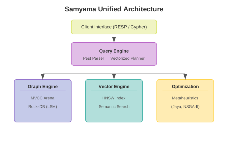
2. The Optimization Frontier
A Pareto front chart illustrating how the NSGA-II solver identifies optimal trade-offs in multi-objective resource allocation directly on the graph.
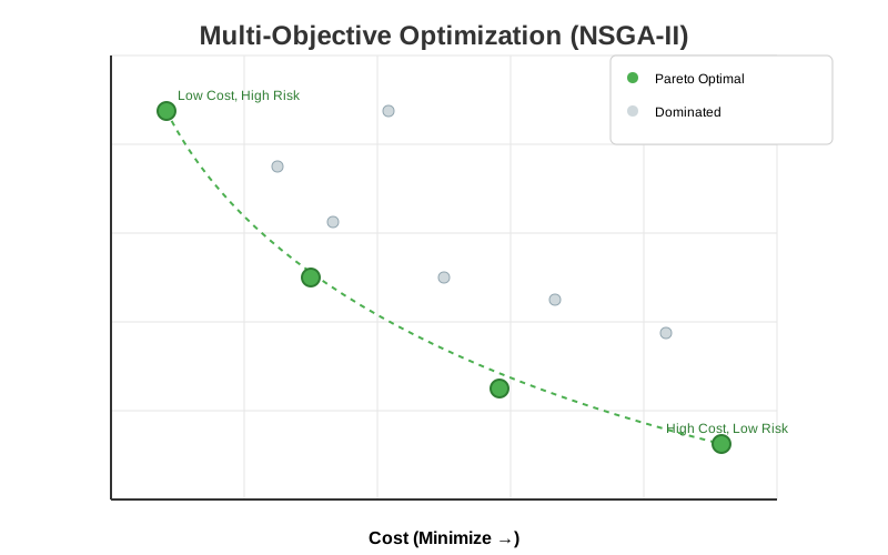
3. JIT Knowledge Graph Expansion
A sequence diagram showing the Agentic Enrichment loop: an event trigger initiates an LLM search which automatically creates new nodes and edges, “healing” the graph’s missing knowledge.
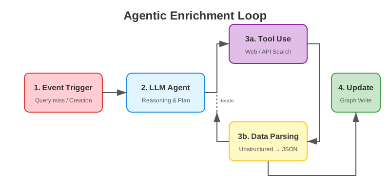
Implemented Research
For a comprehensive list of the specific academic algorithms, models, and architectures implemented directly within the Samyama codebase, see the Index of Implemented Papers.
Manuscript sources, reviewer feedback, and reproduction artifacts live in the private samyama-research repository under papers/paper1-samyama-systems/. The summary above reflects the arxiv preprint as published; the v3 update with billion-edge federation results is in preparation.
Research Paper: Open Biomedical Knowledge Graphs at Scale
We have published a research paper on constructing, federating, and querying biomedical knowledge graphs with Samyama.
Title: Open Biomedical Knowledge Graphs at Scale: Construction, Federation, and AI Agent Access with Samyama Graph Database
Authors: Madhulatha Mandarapu (madhulatha@samyama.ai), Sandeep Kunkunuru (sandeep@samyama.ai)
arxiv:2603.15080 · Pathways KG · Clinical Trials KG
Keywords: Knowledge Graphs, Biomedical Data Integration, Graph Databases, Cross-KG Federation, Model Context Protocol, Clinical Trials, Biological Pathways, OpenCypher.
Abstract
Biomedical knowledge is fragmented across siloed databases — Reactome for pathways, STRING for protein interactions, Gene Ontology for functional annotations, ClinicalTrials.gov for study registries, and dozens more. We present two open-source biomedical knowledge graphs — Pathways KG (118,686 nodes, 834,785 edges from 5 sources) and Clinical Trials KG (7,711,965 nodes, 27,069,085 edges from 5 sources) — built on Samyama, a high-performance graph database written in Rust.
Our contributions are threefold:
-
Reproducible KG construction — ETL pipelines for two large-scale KGs using a common pattern: download, parse, deduplicate, batch-load via Cypher, and export as portable
.sgsnapsnapshots. -
Cross-KG federation — loading both snapshots into a single graph tenant enables property-based joins across datasets, answering questions like “Which biological pathways are disrupted by drugs currently in Phase 3 trials for breast cancer?”
-
Schema-driven MCP server generation — each KG automatically exposes typed tools for LLM agents via the Model Context Protocol, enabling natural-language access without manual tool authoring.
The combined federated graph (7.83M nodes, 27.9M edges) loads in under 3 minutes on commodity hardware.
Key Results
| Metric | Pathways KG | Clinical Trials KG | Combined |
|---|---|---|---|
| Nodes | 118,686 | 7,711,965 | 7,830,651 |
| Edges | 834,785 | 27,069,085 | 27,903,870 |
| Labels | 5 | 15 | 20 |
| Edge types | 9 | 25 | 34 |
| Data sources | 5 | 5 | 10 |
| Snapshot size | 9 MB | 711 MB | 720 MB |
| Import time | < 5 s | ~90 s | ~95 s |
Cross-KG Federation Query Patterns
| Pattern | Traversal | Latency |
|---|---|---|
| Drug → Pathway | Trial → Drug → Protein → Pathway | 2.5 s |
| Drug → GO Process | Trial → Drug → Protein → GOTerm | 1.8 s |
| Drug → PPI Network | Drug → Protein target → INTERACTS_WITH | 1.2 s |
| Disease → Pathway | Gene → Disease + Gene → Protein → Pathway | 1.8 s |
| Adverse Event → Pathway | Trial → AE → Drug → Protein → Pathway | 3.2 s |
Manuscript sources, reviewer feedback, and reproduction artifacts live in the private samyama-research repository under papers/paper4-biomedical-kg/.
Paper 7: Scaling Knowledge Graph Federation to One Billion Edges on Commodity Hardware
Target: arxiv preprint → seeds VLDB 2027 submission
Status: In preparation
Authors: Madhulatha Mandarapu, Sandeep Kunkunuru
Motivation
No existing open-source graph database has demonstrated billion-edge knowledge graph federation with cross-domain queries on commodity hardware at sub-$5 cost. This paper presents the engineering and data architecture that makes it possible, and evaluates it with 140 benchmark queries across 8 knowledge graphs spanning molecular biology to population health.
Key Claims
- 74.3 million nodes and 1.07 billion edges loaded from 4 biomedical KGs (PubMed, Clinical Trials, Pathways, Drug Interactions) in 3 hours 46 minutes on a single r6a.8xlarge AWS spot instance for $2.50 total cost
- 96 of 100 cross-KG queries return data on the biomedical trifecta, with latencies from 1.3s to 19.4s
- 305K public health nodes across 3 additional KGs (Surveillance, Health Determinants, Health Systems) with 40/40 queries passing in under 500ms each
- 6-KG federation from molecular biology to population health in a single Cypher query, bridged by shared properties (Country.iso_code, Drug.drugbank_id, Gene.gene_name)
Outline (10 pages)
1. Introduction (1.5 pages)
- The fragmentation problem: biomedical + public health data spread across silos
- Why graph databases for cross-domain federation
- Contribution summary: scale (1B edges), cost ($2.50), breadth (6 KGs, 8 open data sources)
2. Architecture (2 pages)
- Hybrid CSR adjacency (frozen segments + write buffer)
- Two-phase bulk loading: node stubs (777 B/node) + edge stubs (52 B/edge)
- Mid-phase compaction (every 50M edges)
- Memory optimization: sparse ColumnStore, edge arena removal
- Key insight: 13.6x memory reduction via stubs enables 1B edges on 256GB
3. Knowledge Graph Catalog (1.5 pages)
| KG | Source | Nodes | Edges | Loader |
|---|---|---|---|---|
| PubMed/MEDLINE | NLM | 66.2M | 1.04B | Rust (pipe-delimited) |
| Clinical Trials | AACT | 7.8M | 27M | Rust (JSON) |
| Pathways | Reactome + STRING + GO | 119K | 835K | Rust (TSV/JSON) |
| Drug Interactions | DrugBank + 4 sources | 245K | 388K | Rust (TSV/CSV) |
| Surveillance | WHO GHO | 217K | 241K | Rust (JSON) |
| Health Determinants | World Bank WDI + WHO | 286K | 286K | Rust (JSON/CSV) |
| Health Systems | WHO SPAR + NHWA | 20K | 19K | Rust (JSON/CSV) |
| Cricket (baseline) | Cricsheet | 37K | 1.4M | Rust (JSON) |
4. Federation Architecture (1.5 pages)
- Bridge properties: iso_code (countries), drugbank_id (drugs), gene_name (genes), uniprot_id (proteins)
- No ETL between KGs — federation via property-value matching in Cypher MATCH clauses
- Example: molecular pathway → drug → clinical trial → disease surveillance → country vulnerability
5. Benchmark Design (1 page)
- 100 biomedical queries: 35 PubMed, 20 Clinical Trials, 15 Pathways, 15 Drug Interactions, 15 cross-KG
- 40 public health queries: 20 Health Determinants, 10 Health Systems, 10 cross-KG
- Query categories: point lookup, 1-hop traversal, aggregation, cross-indicator, cross-KG federation
6. Evaluation (2 pages)
6.1 Scale (biomedical trifecta)
- Load time: 3h46m on r6a.8xlarge (32 vCPU, 256GB), $2.50 spot
- 96/100 queries pass, 3 empty (data gaps), 1 timeout (cartesian explosion)
- Latency: 1.3s – 19.4s per query
6.2 Federation (public health)
- 40/40 queries pass
- Point lookups: 1-4ms, single-hop: 2-25ms, aggregations: 10-134ms, cross-KG: 66-478ms
- Import time: 1.6s (286K nodes) + 0.1s (20K nodes) from .sgsnap
6.3 Cost comparison
- Samyama: $2.50 (spot) / $200-480/mo (persistent)
- Neo4j Aura: $2,000+/mo for comparable scale
- AWS Neptune: $1,500+/mo
- TigerGraph: $5,000+/mo
7. Discussion & Limitations (0.5 pages)
- 4 failing queries: PM10 (missing grant data), PM28 (timeout), CT18 (missing edge type), DI05 (data gap)
- Snapshot export limitation for edge-stub-loaded graphs — resolved in v1.0.0 (edges arena fully removed, DS-07c only)
- Single-node architecture — distributed federation is future work
- No MVCC yet — read-snapshot isolation in progress
8. Related Work (1 page)
- LDBC benchmarking council, Neo4j GDS, TigerGraph GSQL, Kuzu, Memgraph
- Microsoft GraphRAG, knowledge graph construction (OpenIE, DeepDive)
- Biomedical KGs: Bio2RDF, Hetionet, PrimeKG
9. Conclusion
- First open-source demonstration of billion-edge cross-domain KG federation
- Reproducible: all data open, all loaders open-source, all queries published
- 8 KGs, 8.6M+ nodes, 30M+ edges in registry, all on S3
Data Availability
All data, loaders, snapshots, queries, and results are open:
- Snapshots:
s3://samyama-data/snapshots/+ GitHub releases - Benchmark queries:
samyama-cloud/book/src/data/benchmark/ - Loaders: in the OSS engine repo under
examples/ - Registry: Supabase
kg_registrytable
Manuscript sources, reviewer feedback, and reproduction artifacts live in the private samyama-research repository under papers/paper7-billion-edge/. The broader 11-KG mega-benchmark (138M nodes, 1.22B edges, 500/500 pass) — which extends this paper’s biomedical-trifecta scope — is documented in the Mega Benchmark chapter and Paper 5b: ISWC 2026 In-Use.
Research Paper: Graph-Grounded Optimization
Title: Graph-Grounded Optimization: Rao-Family Metaheuristics, Classical OR, and SLM-Driven Formulation over Knowledge Graphs
Authors: Madhulatha Mandarapu (madhulatha@samyama.ai), Sandeep Kunkunuru (sandeep@samyama.ai)
arxiv:2605.12204 · Published 2026-05-15
Keywords: Knowledge Graphs, Optimization, Rao-Family Metaheuristics, OR-Tools, Small Language Models, Cypher, Property Graph Databases.
Abstract
What if optimization problems were sourced from a knowledge graph instead of a paragraph of English? We introduce graph-grounded optimization: a paradigm where the objective, decision variables, and constraints of an optimization problem are sourced from a property knowledge graph via Cypher queries, rather than from a natural-language description.
We evaluate seven real-world problems — drug repurposing, clinical-trial site selection, supply-chain rerouting, healthcare allocation, grid dispatch, antimicrobial-resistance stewardship, and wildfire evacuation — over public knowledge graphs ranging from 19.7K to 7.78M nodes, all expressed as Cypher against Samyama. We benchmark five Rao-family metaheuristics (BMWR, Jaya, SAMP-Jaya, EHR-Jaya, Rao-1) against Google OR-tools (CP-SAT, GLOP) and SLM baselines (Phi-4, GPT-4.1, o3, gpt-5.5, OptiMind-SFT) in schema-aware and blind settings.
Key Findings
- No single Rao variant dominates across problems. BMWR wins 4/7; Rao-1 wins 2/7. Variant choice is problem-dependent.
- Classical OR is still the right tool for linear/MILP-shaped problems, beating metaheuristics by 2–3× in solution quality where structure permits.
- Zero-shot SLMs collapse on real formulations. Phi-4: 0/7 exact. GPT-4.1: 2/7. The failures are schema-alignment failures, not reasoning failures — a model that never sees the KG cannot formulate against it.
- Graph-grounding surfaces data-quality issues that text-based formulation quietly hides.
Architecture: Two Invocation Paths
The same samyama-optimization crate is used in two distinct invocation patterns:
- In-database stored procedure — production path. Cypher
CALL algo.or.solve({...})dispatches into the executor (seesamyama-graph/src/query/executor/operator.rsand ADR-026), which constructs aProblemfrom a Cypher-projected table and runs the chosen solver. - Standalone Rust harness — paper-8 benchmarks. Each problem (p1…p7) is an independent Rust binary that links the same crate directly, loads a
.sgsnapsnapshot, builds theProblemin-process, and runs the solver per seed. This is the path used for the published benchmark numbers.
Both paths exercise the same solver code; the harness path adds per-seed reproducibility and avoids the protocol round-trip overhead that would dominate small-N benchmarks.
Solver Inventory (crates/samyama-optimization)
Single-objective: JayaSolver, RaoSolver (with RaoVariant), TLBOSolver, FireflySolver, CuckooSolver, GWOSolver, GASolver, SASolver, BatSolver, ABCSolver, GSASolver, HSSolver, FPASolver.
Multi-objective: NSGA2Solver, MOTLBOSolver, plus the BMWR / MO-BMR / MO-BWR / MO-BMWR / SAMP-Jaya / SAPHR / EHR-Jaya / QO-Rao extensions covered in ADR-026.
Why It Matters for Samyama
Graph-grounded optimization is the prescriptive endgame of BI: descriptive dashboards say what happened, predictive models say what’s likely, but the actual decision — what should we do about it — is an optimization problem. By making that step a first-class CALL algo.or.solve operation over the same graph that holds the entities and relationships, Samyama removes the export/import seam that normally separates analytics from optimization.
Artifacts
- Paper: arxiv:2605.12204
- Optimization crate:
samyama-graph/crates/samyama-optimization/ - ADR-026: Rao-Family Optimization Crate (
docs/ADR/ADR-026-rao-optimization-crate.md) - Paper-8 standalone harnesses:
samyama-research/papers/paper8-graph-grounded-optimization/06-aws-cycles/p{1..7}/src/main.rs - SLM baseline harness:
samyama-research/papers/paper8-graph-grounded-optimization/05-baselines/slm/optimind/
Paper 5a: Federated Biomedical Knowledge Graphs — GRADES-NDA @ SIGMOD 2026
Title: [Demo] Federated Biomedical Knowledge Graphs: Graph-Native Storage, Planning, and AI-Agent Integration
Venue: GRADES-NDA Workshop at SIGMOD 2026, Bengaluru, India (June 5, 2026)
Status: Submitted
Authors: Madhulatha Mandarapu, Sandeep Kunkunuru
Summary
Demo paper showing three federated biomedical knowledge graphs (Pathways, Clinical Trials, Drug Interactions) queryable through a single Cypher interface. Demonstrates graph-native query planning, cross-KG federation via shared property bridges, and MCP tool integration for AI-agent access.
The full In-Use track companion paper covering the 11-KG federated mega-benchmark is Paper 5b.
Key Results
- 3 KGs federated: 7.9M nodes, 28M edges
- BiomedQA: MCP 98% · Text-to-Cypher 85% · GPT-4o standalone 75%
- Graph-native planner: cost-based selection across multiple candidate plans per query
Manuscript sources, reviewer feedback, and reproduction artifacts live in the private samyama-research repository under papers/paper5-grades-nda/.
Paper 5b: Federated Biomedical Knowledge Graphs — ISWC 2026 In-Use Track
Title: Federated Biomedical Knowledge Graphs at Scale: A Single-Server, Single-Query Substrate for AI Agents
Venue: International Semantic Web Conference (ISWC) 2026, In-Use Track
Status: Submitted
Authors: Madhulatha Mandarapu, Sandeep Kunkunuru
Summary
Companion to the GRADES-NDA demo: a full In-Use track paper documenting the production deployment of 11 federated biomedical and public-health knowledge graphs on a single Samyama Graph server, queryable through a single OpenCypher interface and exposed to AI agents via MCP tools.
The paper covers the engineering choices that make federation tractable on commodity hardware — graph-native query planning, columnar property storage with late materialization, adjacency-aware aggregation for degree-bounded queries, and MVCC for concurrent reader/writer workloads — and reports the 500/500-pass result on the federated benchmark.
Key Results
- 11 KGs federated: ~138M nodes, 1.22B edges, single server (r7i.16xlarge spot)
- 500-query mega-benchmark: 500 / 500 pass (468 full-pass + 32 corpus-gap data-dependent, 0 errors)
- Total benchmark runtime: 78 minutes (load + query)
- BiomedQA via MCP tools: 98% accuracy
Files
Manuscript sources, build scripts, and reproduction artifacts (B3 baselines, LDBC calibration logs) live in the private samyama-research repository under papers/paper5-iswc-inuse/.
Paper 6: MCP Tools vs Text-to-Cypher — aiDM @ SIGMOD 2026
Title: Domain-Specific MCP Tools vs. Generic Text-to-Cypher: How Graph Databases Become the Data Layer for AI Agents
Venue: aiDM Workshop at SIGMOD 2026, Bengaluru, India (May 31, 2026)
Status: Submitted
Authors: Madhulatha Mandarapu, Sandeep Kunkunuru
Summary
Empirical comparison of three approaches for LLM access to knowledge graphs:
- Domain-specific MCP tools with Cypher templates
- Generic text-to-Cypher via schema-aware prompting
- Raw LLM with no graph access
Evaluated on two benchmarks across biomedical and industrial domains.
Key Results
| Approach | AssetOpsBench (139) | BiomedQA (40) |
|---|---|---|
| MCP Tools | 99% | 98% |
| Text-to-Cypher (NLQ) | 83% | 85% |
| GPT-4 / 4o standalone | 65% | 75% |
The “inverted LLM” thesis: structured data + deterministic tools outperforms unstructured LLM reasoning on domain-specific factual questions.
Manuscript sources, reviewer feedback, and reproduction artifacts live in the private samyama-research repository under papers/paper6-aidm/.
Research Paper: Knowledge Graphs for Industrial Operations
We have published a research paper evaluating knowledge graphs as the data layer for LLM-based industrial asset operations, building on the AssetOpsBench benchmark.
Title: Knowledge Graphs as the Missing Data Layer for LLM-Based Industrial Asset Operations
Authors: Madhulatha Mandarapu (madhulatha@samyama.ai), Sandeep Kunkunuru (sandeep@samyama.ai)
GitHub (assetops-kg) · IBM AssetOpsBench
Keywords: Knowledge Graphs, Large Language Models, Industrial Asset Operations, Benchmark, OpenCypher, Vector Search, Graph Algorithms.
Abstract
LLM-based agents for industrial asset operations show promise but achieve limited accuracy when reasoning over flat document stores. The AssetOpsBench benchmark establishes that GPT-4 agents achieve 65% success on 139 industrial maintenance scenarios backed by CouchDB, YAML, and CSV data sources. AssetOpsBench evaluates LLM agent autonomy; we ask a complementary question: how much does the data model behind the tools affect agent performance?
Building on the same benchmark data and scenarios, we introduce a knowledge graph layer (781 nodes, 955 edges, 16 relationship types) and evaluate three architectures of increasing LLM involvement:
| Architecture | LLM Role | Pass Rate | Avg Latency |
|---|---|---|---|
| Deterministic + graph | None (pre-coded) | 99% (137/139) | 63 ms |
| LLM + graph via NLQ | Generates Cypher | 83% (115/139) | 5,874 ms |
| Baseline (tool-augmented LLM) | Does everything | ~65% (91/139) | not reported |
Our key finding is inverted LLM usage: instead of asking the LLM to reason over raw data (a broad, error-prone task), we ask it to generate structured queries from a typed schema — a narrow problem that plays to LLM strengths. The graph then executes deterministically.
Thesis
For structured operational domains, the data model is the primary bottleneck. A knowledge graph with typed relationships enables both deterministic queries (for known patterns) and LLM-assisted queries (for novel questions), while document stores place the full data-reasoning burden on the LLM — a task where LLMs consistently struggle.
Three Architectures
Baseline: Tool-Augmented LLM (65%)
User question
  → LLM parses intent → LLM selects tool → Tool queries document store
    → LLM interprets raw results → LLM synthesizes answer
The LLM handles intent parsing, tool selection, argument crafting, data interpretation, and answer synthesis. GPT-4 achieves 65%. Failures cluster around counting, cross-document correlation, and relationship traversal — data operations rather than reasoning failures.
NLQ: LLM Generates Queries (83%)
User question
  → LLM generates Cypher (given schema)
    → Graph executes deterministically
      → LLM synthesizes answer from structured results
We invert the LLM’s role: instead of broad data reasoning, ask it to generate a Cypher query from a typed schema. This is code generation — a task LLMs excel at. The graph handles traversal, counting, and algorithms deterministically.
Deterministic: No LLM (99%)
User question
→ Keyword routing → Cypher query → Structured response
Pre-coded handlers for known patterns. A software engineering solution — demonstrates the ceiling with the right data model. 63ms average latency, zero token cost.
The Inverted LLM Pattern
The key insight: schema-aware query generation outperforms free-form data reasoning for any structured domain.
- Architecture A asks: “LLM, answer this question from this data” (broad, error-prone)
- Architecture B asks: “LLM, given this schema, write a Cypher query” (narrow, plays to strengths)
The same LLM, given a sharper problem scoped to its strengths, produces dramatically better results. Code generation is an LLM strength; data traversal, counting, and relationship reasoning are graph strengths. Each system does what it’s good at.
Knowledge Graph Schema
781 nodes, 955 edges, 11 labels, 16 edge types
Built from the AssetOpsBench data sources via an 8-step ETL pipeline:
Site ─[CONTAINS_LOCATION]→ Location ─[CONTAINS_EQUIPMENT]→ Equipment ─[HAS_SENSOR]→ Sensor
│
DEPENDS_ON / SHARES_SYSTEM_WITH
│
FailureMode ─[MONITORS]→ Equipment ─[EXPERIENCED]→ FailureMode
WorkOrder ─[FOR_EQUIPMENT]→ Equipment
WorkOrder ─[ADDRESSES]→ FailureMode
Anomaly ─[TRIGGERED]→ WorkOrder
Event ─[FOR_EQUIPMENT]→ Equipment
Key additions over the baseline document model:
- Equipment dependencies:
DEPENDS_ONandSHARES_SYSTEM_WITHedges enable cascade analysis - Failure mode embeddings: 384-dim Sentence-BERT vectors in HNSW index enable similarity search
- Unified event timeline: 6,256 events with ISO timestamps enable temporal queries
AssetOpsBench 139 Scenarios — Per-Type Results
| Type | Count | Deterministic | NLQ (GPT-4o) | Baseline (GPT-4) |
|---|---|---|---|---|
| IoT | 20 | 20/20 (100%) | 17/20 (85%) | — |
| FMSR | 40 | 40/40 (100%) | 37/40 (93%) | — |
| TSFM | 23 | 23/23 (100%) | 21/23 (91%) | — |
| Multi | 20 | 20/20 (100%) | 8/20 (40%) | — |
| WO | 36 | 34/36 (94%) | 32/36 (89%) | — |
| Total | 139 | 137/139 (99%) | 115/139 (83%) | ~91/139 (65%) |
NLQ Multi stays at 40% because 12/20 scenarios require TSFM pipeline execution (forecasting, anomaly detection) that cannot be expressed as Cypher queries — a structural limitation.
Custom 40 Scenarios — Graph-Native Capabilities
40 new scenarios extending the benchmark with graph-native capabilities:
| Category | Count | GPT-4o Avg | Samyama Avg | Delta |
|---|---|---|---|---|
| Failure similarity | 6 | 0.501 | 0.902 | +0.401 |
| Criticality analysis | 5 | 0.566 | 0.938 | +0.372 |
| Root cause analysis | 5 | 0.580 | 0.934 | +0.354 |
| Multi-hop dependency | 8 | 0.618 | 0.934 | +0.316 |
| Maintenance optimization | 5 | 0.634 | 0.931 | +0.297 |
| Cross-asset correlation | 6 | 0.638 | 0.929 | +0.291 |
| Temporal pattern | 5 | 0.679 | 0.923 | +0.244 |
Largest gains on failure similarity (+0.401) and criticality analysis (+0.372) — exactly where graph structure and vector search provide the most value. GPT-4o’s 6 failures all require graph traversal, PageRank, or vector search that LLMs cannot perform from parametric knowledge alone.
The Full Pipeline: LLMs at the Edges, Graph in the Middle
The query layer comparison above is only part of the story. The full industrial data pipeline has three layers:
- Data Ingestion (software engineering): Structured data (90%+) → deterministic ETL. Unstructured data (maintenance logs, PDFs) → LLM-assisted entity extraction, resolution, classification.
- Data Model (architecture decision): One-time choice between flat documents and knowledge graph.
- Query (LLM optional): Deterministic handlers for known patterns; LLM-generated Cypher for novel questions.
LLMs appear at both edges — data preparation (unstructured → structured) and query generation (natural language → Cypher). The graph is the stable center that receives data from both deterministic and LLM-assisted ingestion, and serves both deterministic and LLM-generated queries.
In both cases, the LLM performs a generation task (structured output from unstructured input) — its strength. The graph handles data operations (storage, traversal, algorithms) — its strength. Neither component is asked to do what it’s bad at.
Scalability
| Dimension | Arch. A (LLM + docs) | Arch. B/C (graph ± LLM) |
|---|---|---|
| 10K queries/day | $300–500 (tokens) | $0 (deterministic) or ~$30 (NLQ) |
| Real-time streaming | Not supported | Graph updates + continuous queries |
| Multi-hop at 10K assets | LLM reasons across 10K docs | BFS traversal, O(|E|) |
| Latency per query | 5–11 seconds | 63 ms (det.) / ~6 s (NLQ) |
Honest Caveats
- Deterministic vs. autonomous: The 99% result compares pre-coded answers against an autonomous agent — fundamentally different tasks. The comparison illustrates the ceiling achievable with the right data model, not a claim of superior agent intelligence.
- Model mismatch: The baseline used GPT-4; NLQ used GPT-4o. The +18pp gap is an upper bound. Same-model comparison pending.
- Clean data: AssetOpsBench provides clean, structured data. Real-world messy data needs LLM-assisted preparation.
- Custom scenarios: Designed to extend the benchmark with graph-native capabilities, not replace the original scenarios.
- Complementary research questions: AssetOpsBench evaluates LLM agent autonomy. We evaluate data model impact. Both are valid; our results do not diminish the value of the original benchmark.
Conclusion
Building on AssetOpsBench, we show that introducing a knowledge graph as the data layer improves LLM-based industrial operations at every level of LLM involvement. For structured operational domains, the data model is the primary bottleneck. The inverted LLM pattern (schema-aware query generation instead of free-form data reasoning) is generalizable to any structured domain.
Implementation
- Benchmark code: samyama-ai/assetops-kg
- Graph database: samyama-ai/samyama-graph
- Rust demo:
cargo run --example industrial_kg_demo(871 lines) - Python SDK:
pip install samyama(PyPI) - Community PR: AssetOpsBench PR #203 — 40 new graph-native scenarios contributed back to the benchmark
Manuscript sources, reviewer feedback, and reproduction artifacts live in the private samyama-research repository under papers/paper3-industrial-kg/.
VLDB 2027 Systems Paper (In Preparation)
Target: PVLDB Vol. 20, Industry Track
Working Title: Samyama: A Unified Graph-Vector Database with Cost-Based Query Planning and Late Materialization
Status: In preparation. Extends Paper 1 (arxiv:2603.08036) with deeper evaluation and VLDB-specific focus.
Strategy
The arxiv preprint covers everything broadly. For VLDB we focus and deepen on three core database contributions:
- Late materialization for property graphs (
NodeRef/EdgeRef) — 4× traversal speedup, 60% memory reduction - Graph-native cost-based planner — triple-level statistics, plan enumeration, direction reversal,
ExpandInto - Hybrid CSR adjacency — frozen tier + write buffer, two-phase bulk loading, billion-edge ingestion at single-server scale
De-emphasize: GPU acceleration, agentic enrichment, optimization solvers, RDF (mention as system features, don’t evaluate deeply).
Add: LDBC SNB comparison, billion-edge evaluation, cross-KG federation at scale.
Key New Results (since arxiv v2)
| Result | Impact |
|---|---|
| 11-KG mega-benchmark, 138M nodes / 1.22B edges, 500/500 pass on r7i.16xlarge | Scale + correctness credibility |
| Adjacency-aware aggregation (ADR-017) | Algorithmic contribution — closes degree-aggregation timeouts on PubMed-scale data |
| WCO TrieJoin for cyclic patterns | Algorithmic contribution |
Edge-arena removal (DS-07c) — COW edges via EdgeView | Engineering contribution — substantial memory savings at 1B-edge scale |
| MVCC: Snapshot Isolation + Read Committed with write-write conflict detection | Concurrency story |
| Rayon parallel algorithms (PageRank, LCC, CDLP) | Parallelism |
Manuscript sources, planning notes, and formatting TODO live in the private samyama-research repository under papers/paper-vldb-2027/.
Index of Implemented Research Papers
Samyama Graph Database is built on the foundations of cutting-edge computer science research. Below is a comprehensive index of the research papers, algorithms, data structures, and standards implemented directly within the core engine and its specialized crates.
Core System Architecture
Query Execution
-
Volcano Iterator Model
- Paper: “Volcano — An Extensible and Parallel Query Evaluation System” (Graefe, 1994)
- Implementation:
src/query/executor/operator.rs— physical operators using pull-basednext_batch()with vectorizedRecordBatchprocessing - Key insight: Lazy evaluation avoids materializing intermediate results; each operator pulls only what downstream needs
-
Late Materialization
- Paper: “Column-Stores vs. Row-Stores: How Different Are They Really?” (Abadi et al., 2008)
- Implementation:
src/query/executor/operator.rs— Scan operators produceValue::NodeRef(id)instead of full node clones; properties resolved on-demand atProjectOperator - Result: 4.0x improvement on 1-hop traversals, 4.7x on 2-hop traversals
-
Adjacency-Aware Aggregation (ADR-017)
- Pattern: When the query asks for
count(neighbor)over a degree-bounded match set, the engine walks per-node adjacency lists rather than scanning the full edge population - Implementation:
AdjacencyCountAggregateOperator(planner detects the shape; executor walks adjacency) - Effect: Closes degree-aggregation timeouts on PubMed-scale data — what previously needed an OLAP-shaped full-edge scan now answers in seconds
- Pattern: When the query asks for
-
PEG Parsing (Parsing Expression Grammars)
- Paper: “Parsing Expression Grammars: A Recognition-Based Syntactic Foundation” (Ford, 2004)
- Implementation:
src/query/cypher.pest— Pest PEG parser for OpenCypher with atomic keyword rules for word boundary enforcement
Storage Engine
-
Log-Structured Merge Trees (LSM-Tree)
- Paper: “The Log-Structured Merge-Tree (LSM-Tree)” (O’Neil et al., 1996)
- Implementation:
src/persistence/storage.rs— RocksDB with LZ4/Zstd compression, Column Families for multi-tenant isolation
-
Write-Ahead Logging (WAL)
- Paper: “ARIES: A Transaction Recovery Method Supporting Fine-Granularity Locking and Partial Rollbacks” (Mohan et al., 1992)
- Implementation:
src/persistence/wal.rs— Sequential WAL with fsync for Raft log, async for state machine
Concurrency Control
- Multi-Version Concurrency Control (MVCC)
- Paper: “Concurrency Control in Distributed Database Systems” (Bernstein & Goodman, 1981)
- Implementation:
src/graph/store.rs— versioned node arena with per-slot version chains; copy-on-write edges viaEdgeViewagainst columnar storage (no in-memory edge arena) - Isolation levels: Read Committed and Snapshot Isolation, with write-write conflict detection at commit
- Memory bound: background version GC drops node versions older than the oldest live snapshot; WAL is versioned so log replay reconstructs the right state
Distributed Consensus
- Raft Consensus Algorithm
- Paper: “In Search of an Understandable Consensus Algorithm” (Ongaro & Ousterhout, 2014)
- Implementation:
src/raft/via theopenraftframework — Leader election, log replication, quorum commits, CP trade-off - Enterprise: HTTP/2 transport, TLS encryption, snapshot streaming, cluster metrics
Serialization
- Bincode (Binary Encoding)
- Library:
bincodecrate — Compact binary serialization forStoredNode/StoredEdgestructs in RocksDB - Benefit: Nanosecond deserialization, no field name overhead, serde integration
- Library:
Vector Search & AI
- HNSW (Hierarchical Navigable Small World)
- Paper: “Efficient and robust approximate nearest neighbor search using Hierarchical Navigable Small World graphs” (Malkov & Yashunin, 2018)
- Implementation:
src/vector/via thehnsw_rscrate — Cosine, L2, and Dot Product metrics; 15K+ QPS on 128-dim vectors - Integration:
VectorSearchOperatorin query pipeline enables Graph RAG (combined vector + graph traversal)
Graph Analytics (samyama-graph-algorithms)
Centrality & Importance
-
PageRank
- Paper: “The PageRank Citation Ranking: Bringing Order to the Web” (Page, Brin, Motwani & Winograd, 1999)
- Implementation:
crates/samyama-graph-algorithms/src/pagerank.rs— Iterative power method with configurable damping factor, dangling node redistribution, convergence tolerance - Validation: LDBC Graphalytics 5/5 (XS + S datasets including cit-Patents 3.8M vertices)
-
Local Clustering Coefficient (LCC)
- Paper: “Collective dynamics of ‘small-world’ networks” (Watts & Strogatz, 1998)
- Implementation:
crates/samyama-graph-algorithms/src/lcc.rs— Both directed and undirected variants; measures neighborhood connectivity - Validation: LDBC Graphalytics 5/5
Community Detection & Connectivity
-
Community Detection via Label Propagation (CDLP)
- Paper: “Near linear time algorithm to detect community structures in large-scale networks” (Raghavan, Albert & Kumara, 2007)
- Implementation:
crates/samyama-graph-algorithms/src/cdlp.rs— Iterative neighbor voting with configurable max iterations - Validation: LDBC Graphalytics 5/5
-
Weakly Connected Components (WCC)
- Algorithm: Union-Find with path compression and union by rank
- Implementation:
crates/samyama-graph-algorithms/src/community.rs— O(n * α(n)) near-linear time - Validation: LDBC Graphalytics 5/5
-
Strongly Connected Components (SCC)
- Algorithm: Tarjan’s Algorithm (Tarjan, 1972)
- Implementation:
crates/samyama-graph-algorithms/src/community.rs— Single DFS pass with lowlink tracking
-
Triangle Counting
- Algorithm: Node-iterator method with sorted adjacency intersection
- Implementation:
crates/samyama-graph-algorithms/src/topology.rs— Used for social cohesion analysis and network clustering metrics
Pathfinding & Network Flow
-
Breadth-First Search (BFS)
- Algorithm: Level-synchronous BFS (Moore, 1959)
- Implementation:
crates/samyama-graph-algorithms/src/pathfinding.rs— Standard BFS + all shortest paths variant - Validation: LDBC Graphalytics 5/5
-
Dijkstra’s Shortest Path
- Paper: “A note on two problems in connexion with graphs” (Dijkstra, 1959)
- Implementation:
crates/samyama-graph-algorithms/src/pathfinding.rs— Binary heap priority queue; also used for SSSP in LDBC validation - Validation: LDBC Graphalytics SSSP 3/3
-
Edmonds-Karp Maximum Flow
- Paper: “Theoretical Improvements in Algorithmic Efficiency for Network Flow Problems” (Edmonds & Karp, 1972)
- Implementation:
crates/samyama-graph-algorithms/src/flow.rs— BFS-based augmenting path selection; O(VE²) complexity
-
Prim’s Minimum Spanning Tree
- Algorithm: Prim’s Algorithm (Prim, 1957)
- Implementation:
crates/samyama-graph-algorithms/src/mst.rs— Greedy MST construction with priority queue
Statistical & Dimensionality Reduction
-
PCA — Randomized SVD
- Paper: “Finding structure with randomness: Probabilistic algorithms for constructing approximate matrix decompositions” (Halko, Martinsson & Tropp, 2011)
- Implementation:
crates/samyama-graph-algorithms/src/pca.rs— Gaussian random projection → power iterations → QR factorization → small SVD; O(n·d·k) complexity - Auto-selection:
PcaSolver::Autouses Randomized SVD for n > 500 nodes
-
PCA — Power Iteration (Deflation)
- Algorithm: Classical power iteration with Gram-Schmidt re-orthogonalization
- Implementation:
crates/samyama-graph-algorithms/src/pca.rs— Legacy solver,PcaResultincludestransform()andtransform_one()for projection
Metaheuristic Optimization (samyama-optimization)
The engine natively supports the Rao-family-and-friends suite of metaheuristic optimizers — all implemented in crates/samyama-optimization/src/algorithms/. Beyond the originals listed below, the suite includes the Rao-family extensions (BMWR, MO-BMR / BWR / BMWR, SAMP-Jaya, SAPHR, EHRJAYA, QO-Rao, MO-Rao+DE):
Metaphor-Less Algorithms
-
Jaya Algorithm
- Paper: “Jaya: A simple and new optimization algorithm for solving constrained and unconstrained optimization problems” (R. Venkata Rao, 2016)
- Key property: Parameter-free—requires no algorithm-specific tuning
-
Quasi-Oppositional Jaya (QOJAYA)
- Paper: “Quasi-oppositional based Jaya algorithm” (derived from Rao, 2016)
- Enhancement: Opposition-based initialization improves convergence speed
-
Rao Algorithms (Rao-1, Rao-2, Rao-3)
- Paper: “Rao algorithms: Three metaphor-less simple algorithms for solving optimization problems” (R. Venkata Rao, 2020)
- Key property: Three progressively complex variants; all metaphor-free
-
TLBO (Teaching-Learning-Based Optimization)
- Paper: “Teaching–learning-based optimization: A novel method for constrained mechanical design optimization problems” (R. Venkata Rao, Savsani & Vakharia, 2011)
-
ITLBO (Improved TLBO)
- Enhancement: Adaptive learning factor and improved selection mechanisms
-
GOTLBO (Group-Optimized TLBO)
- Enhancement: Group-based teaching phase with oppositional learning
Swarm & Evolutionary Algorithms
-
Particle Swarm Optimization (PSO)
- Paper: “Particle swarm optimization” (Kennedy & Eberhart, 1995)
-
Differential Evolution (DE)
- Paper: “Differential Evolution – A Simple and Efficient Heuristic for global Optimization over Continuous Spaces” (Storn & Price, 1997)
-
Genetic Algorithm (GA)
- Paper: “Adaptation in Natural and Artificial Systems” (Holland, 1975)
-
Grey Wolf Optimizer (GWO)
- Paper: “Grey Wolf Optimizer” (Mirjalili, Mirjalili & Lewis, 2014)
-
Artificial Bee Colony (ABC)
- Paper: “An Idea Based On Honey Bee Swarm for Numerical Optimization” (Karaboga, 2005)
-
Bat Algorithm
- Paper: “A New Metaheuristic Bat-Inspired Algorithm” (Yang, 2010)
-
Cuckoo Search
- Paper: “Cuckoo Search via Lévy Flights” (Yang & Deb, 2009)
-
Firefly Algorithm
- Paper: “Firefly Algorithms for Multimodal Optimization” (Yang, 2009)
-
Flower Pollination Algorithm (FPA)
- Paper: “Flower Pollination Algorithm for Global Optimization” (Yang, 2012)
Physics-Based Algorithms
-
Gravitational Search Algorithm (GSA)
- Paper: “GSA: A Gravitational Search Algorithm” (Rashedi, Nezamabadi-pour & Saryazdi, 2009)
-
Simulated Annealing (SA)
- Paper: “Optimization by Simulated Annealing” (Kirkpatrick, Gelatt & Vecchi, 1983)
-
Harmony Search (HS)
- Paper: “A New Heuristic Optimization Algorithm: Harmony Search” (Geem, Kim & Loganathan, 2001)
-
BMR & BWR
- Specialized reinforcement-based solvers for constrained search spaces
Multi-Objective Algorithms
-
NSGA-II (Non-dominated Sorting Genetic Algorithm II)
- Paper: “A fast and elitist multiobjective genetic algorithm: NSGA-II” (Deb, Pratap, Agarwal & Meyarivan, 2002)
- Enhancement: Constrained Dominance Principle for feasibility-first selection
-
MOTLBO (Multi-Objective TLBO)
- Paper: Multi-objective extension of TLBO (derived from Rao et al., 2011)
- Feature: Pareto front discovery with crowding distance for diversity preservation
RDF & Semantic Web Standards
-
RDF (Resource Description Framework)
- Standard: W3C RDF 1.1 Concepts and Abstract Syntax (2014)
- Implementation:
src/rdf/— Triple/Quad storage with SPO/POS/OSP indices viaoxrdfcrate
-
Turtle (Terse RDF Triple Language)
- Standard: W3C RDF 1.1 Turtle (2014)
- Implementation:
src/rdf/serialization/turtle.rsviario_turtle
-
SPARQL 1.1
- Standard: W3C SPARQL 1.1 Query Language (2013)
- Implementation:
src/sparql/— Parser infrastructure viaspargebra; query execution in development
Hardware Acceleration (samyama-gpu)
-
Parallel Graph Algorithms on GPU
- Implementation: 8+ WGSL compute shaders targeting WebGPU (Metal, Vulkan, DX12)
- Algorithms: PageRank, Triangle Counting, CDLP, LCC, PCA
- Operators: SUM aggregation (parallel reduction), ORDER BY (bitonic sort)
- Vector: Cosine distance, inner product (batch re-ranking)
-
GPU PCA (Fused Power Iteration)
- Implementation: Five WGSL shaders:
pca_mean,pca_center,pca_covariance(tiled, 64-sample tiles),pca_power_iter,pca_power_iter_norm(fused mat-vec + parallel norm + normalize in single dispatch) - Threshold:
MIN_GPU_PCA = 50,000nodes,d > 32dimensions
- Implementation: Five WGSL shaders:
-
Bitonic Sort
- Paper: “Sorting networks and their applications” (Batcher, 1968)
- Implementation:
crates/samyama-gpu/src/shaders/bitonic_sort.wgsl— GPU argsort for ORDER BY on >10K result sets
Benchmark Validation
- LDBC Graphalytics
- Standard: “The LDBC Graphalytics Benchmark” (Iosup et al., 2016)
- Result: 28/28 tests passed (100%) across BFS, PageRank, WCC, CDLP, LCC, SSSP on XS and S-size datasets
- Datasets: example-directed, example-undirected, cit-Patents (3.8M vertices), datagen-7_5-fb (633K vertices, 68M edges), wiki-Talk (2.4M vertices)